This content was presented to Nelson\Nygaard Staff at a Lunch and Learn webinar on Thursday, December 9th, 2021, and is available as a recording here and embedded below.
Introduction
This webinar was developed by request to help staff at Nelson\Nygaard understand how typical GIS tasks may be duplicated in R. Ideas for particular tasks were crowdsourced from the #r-users Slack channel. If there are other tasks like this, please list them for Bryan and he can develop another webinar like this one, with these further tasks, at a later date.
Most of the topics discussed today have already been discussed in previous webinars – I will try to link related webinars where relevant. Nevertheless, the goal is to emphasize how these topics are similar to procedures often carried out in ArcGIS.
Agenda
- Refresher on Basics of Spatial Data in R (10 minutes)
- Reading data in from various formats (10 minutes)
- Coordinate systems in R (5 minutes)
- Geometric operations (25 minutes)
- Origin-destination data (10 minutes)
Refresher on Basics of Vector Spatial Data in R
There were previously a variety of other packages for managing spatial data in R, but now the standard package (since 2017 or so) for vector spatial data in R is sf. It is well maintained and intuitive, and there are many other packages built upon the classes and functions implemented within sf.
I am going to refresh a few of the basics below, but I considered this package extensively in a previous webinar to refer to as well. I would also consider the other webinars on this website with the geospatial category tag for further examples, and will link some relevant books and DataCamp courses at the end of the training for further reference.
We are going to focus on vector spatial data today, since that is what sf is set up to deal with. If you need to use raster data, I will refer you to the terra package and hope to do a webinar on this topic in the future.
What is a feature?
A feature is thought of as a thing, or an object in the real world, such as a building or a tree. As is the case with objects, they often consist of other objects. This is the case with features too: a set of features can form a single feature. A forest stand can be a feature, a forest can be a feature, a city can be a feature. A satellite image pixel can be a feature, a complete image can be a feature too.
Features have a geometry describing where on Earth the feature is located, and they have attributes, which describe other properties. The geometry of a tree can be the delineation of its crown, of its stem, or the point indicating its centre. Other properties may include its height, color, diameter at breast height at a particular date, and so on.
The standard says: “A simple feature is defined by the OpenGIS Abstract specification to have both spatial and non-spatial attributes. Spatial attributes are geometry valued, and simple features are based on 2D geometry with linear interpolation between vertices.” We will see soon that the same standard will extend its coverage beyond 2D and beyond linear interpolation. Here, we take simple features as the data structures and operations described in the standard.
Dimensions
All geometries are composed of points. Points are coordinates in a 2-, 3- or 4-dimensional space. All points in a geometry have the same dimensionality. In addition to X and Y coordinates, there are two optional additional dimensions:
- a Z coordinate, denoting altitude
- an M coordinate (rarely used), denoting some measure that is associated with the point, rather than with the feature as a whole (in which case it would be a feature attribute); examples could be time of measurement, or measurement error of the coordinates
The four possible cases then are:
- two-dimensional points refer to x and y, easting and northing, or longitude and latitude, we refer to them as XY
- three-dimensional points as XYZ
- three-dimensional points as XYM
- four-dimensional points as XYZM (the third axis is Z, fourth M)
Simple feature geometry types
The following seven simple feature types are the most common, and are for instance the only ones used for GeoJSON:
| type | description |
|---|---|
POINT |
zero-dimensional geometry containing a single point |
LINESTRING |
sequence of points connected by straight, non-self intersecting line pieces; one-dimensional geometry |
POLYGON |
geometry with a positive area (two-dimensional); sequence of points form a closed, non-self intersecting ring; the first ring denotes the exterior ring, zero or more subsequent rings denote holes in this exterior ring |
MULTIPOINT |
set of points; a MULTIPOINT is simple if no two Points in the MULTIPOINT are equal |
MULTILINESTRING |
set of linestrings |
MULTIPOLYGON |
set of polygons |
GEOMETRYCOLLECTION |
set of geometries of any type except GEOMETRYCOLLECTION |
Each of the geometry types can also be a (typed) empty set, containing zero coordinates (for POINT the standard is not clear how to represent the empty geometry). Empty geometries can be thought of being the analogue to missing (NA) attributes, NULL values or empty lists.
The remaining geometries 10 are rarer, but increasingly find implementations:
| type | description |
|---|---|
CIRCULARSTRING |
The CIRCULARSTRING is the basic curve type, similar to a LINESTRING in the linear world. A single segment requires three points, the start and end points (first and third) and any other point on the arc. The exception to this is for a closed circle, where the start and end points are the same. In this case the second point MUST be the center of the arc, i.e., the opposite side of the circle. To chain arcs together, the last point of the previous arc becomes the first point of the next arc, just like in LINESTRING. This means that a valid circular string must have an odd number of points greater than 1. |
COMPOUNDCURVE |
A compound curve is a single, continuous curve that has both curved (circular) segments and linear segments. That means that in addition to having well-formed components, the end point of every component (except the last) must be coincident with the start point of the following component. |
CURVEPOLYGON |
Example compound curve in a curve polygon: CURVEPOLYGON(COMPOUNDCURVE(CIRCULARSTRING(0 0,2 0, 2 1, 2 3, 4 3),(4 3, 4 5, 1 4, 0 0)), CIRCULARSTRING(1.7 1, 1.4 0.4, 1.6 0.4, 1.6 0.5, 1.7 1) ) |
MULTICURVE |
A MultiCurve is a 1-dimensional GeometryCollection whose elements are Curves, it can include linear strings, circular strings or compound strings. |
MULTISURFACE |
A MultiSurface is a 2-dimensional GeometryCollection whose elements are Surfaces, all using coordinates from the same coordinate reference system. |
CURVE |
A Curve is a 1-dimensional geometric object usually stored as a sequence of Points, with the subtype of Curve specifying the form of the interpolation between Points |
SURFACE |
A Surface is a 2-dimensional geometric object |
POLYHEDRALSURFACE |
A PolyhedralSurface is a contiguous collection of polygons, which share common boundary segments |
TIN |
A TIN (triangulated irregular network) is a PolyhedralSurface consisting only of Triangle patches. |
TRIANGLE |
A Triangle is a polygon with 3 distinct, non-collinear vertices and no interior boundary |
Note that CIRCULASTRING, COMPOUNDCURVE and CURVEPOLYGON are not described in the SFA standard, but in the SQL-MM part 3 standard. The descriptions above were copied from the PostGIS manual.
How simple features in R are organized
Package sf represents simple features as native R objects.
Similar to PostGIS, all functions and methods
in sf that operate on spatial data are prefixed by st_, which
refers to spatial type; this makes them easily findable
by command-line completion. Simple features are implemented as
R native data, using simple data structures (S3 classes, lists,
matrix, vector). Typical use involves reading, manipulating and
writing of sets of features, with attributes and geometries.
As attributes are typically stored in data.frame objects (or the
very similar tbl_df), we will also store feature geometries in
a data.frame column. Since geometries are not single-valued,
they are put in a list-column, a list of length equal to the number
of records in the data.frame, with each list element holding the simple
feature geometry of that feature. The three classes used to
represent simple features are:
sf, the table (data.frame) with feature attributes and feature geometries, which containssfc, the list-column with the geometries for each feature (record), which is composed ofsfg, the feature geometry of an individual simple feature.
For more on details on all this, I defer to the documentation where I copied most of this from!
Reading in Data
sf can read vector geometry data directly from a variety of sources:
- ESRI shapefiles (.shp)
- ESRI geodatabases (.gdb)
- GeoJSON packets (.geojson)
- KML files (.kml)
- PostgreSQL databases using the PostGIS extension
- sf can also assemble geometries on-the-fly from tabular formats as needed (e.g., point geometries from a GTFS stops table)
- Others, I am sure, though these are the common ones I find!
Ultimately, geometries can be developed from scratch within R, though it is more common that you are reading in geometries from some other data source and editing them or using them for analysis in some way.
For the most part, reading is as simple as using the read_sf() function and pointing to the file (or table in a database) you are interested in, though depending on the file type you may need some additional parameters.
Example
In this simple example, I am going to show how simple it is to read various types of spatial data (all describing the the city boundaries within the Portland metropolitan area) into R.
To show what the shapes look like, I am going to use the leaflet package. For a refresher on how to use leaflet, refer to related past webinars or the leaflet documentation.
As I will explain in the next section, spatial data is always relative to a coordinate system. In this case, in order to map it with leaflet, we need to translate the data to the WGS 84 geographic coordinate system. I will do this on the fly in the leaflet call. We will investigate the original data’s coordinate system in the next section.
#Loading in basic packages
library(tidyverse)
library(sf)
library(leaflet)

#Shapefile
city_bounds_shapefile = read_sf("data/shapefiles/City_Boundaries/City_Boundaries.shp")
city_bounds_shapefile
Simple feature collection with 57 features and 5 fields
Geometry type: MULTIPOLYGON
Dimension: XY
Bounding box: xmin: -13747930 ymin: 5632401 xmax: -13606340 ymax: 5800163
Projected CRS: WGS 84 / Pseudo-Mercator
# A tibble: 57 × 6
OBJECTID CITYNAME Shape…¹ Shape…² AREA geometry
<int> <chr> <dbl> <dbl> <dbl> <MULTIPOLYGON [m]>
1 1 Amity 12190. 3.27e6 1.75e7 (((-13715106 5640691, -1…
2 2 Banks 14881. 3.94e6 2.08e7 (((-13704572 5720068, -1…
3 3 Barlow 3500. 2.70e5 1.44e6 (((-13661258 5661614, -1…
4 4 Battle G… 58040. 4.54e7 2.38e8 (((-13640769 5748205, -1…
5 5 Beaverton 220170. 1.04e8 5.49e8 (((-13677135 5707075, -1…
6 6 Camas 89229. 8.32e7 4.38e8 (((-13632612 5725461, -1…
7 7 Canby 47680. 2.44e7 1.30e8 (((-13656620 5667070, -1…
8 8 Carlton 10999. 4.64e6 2.47e7 (((-13713126 5667383, -1…
9 9 Clatskan… 26298. 6.82e6 3.53e7 (((-13714193 5799662, -1…
10 10 Columbia… 10958. 4.19e6 2.18e7 (((-13671542 5764929, -1…
# … with 47 more rows, and abbreviated variable names ¹Shape_Leng,
# ²Shape_Arealeaflet() %>%
addProviderTiles("CartoDB.Positron") %>%
addPolygons(data = city_bounds_shapefile %>% st_transform(4326),
label=~ CITYNAME,
fillOpacity = 0.5,opacity = 1,
color="white",fillColor = "blue",
weight=1)city_bounds_kml = read_sf("data/kml/City_Boundaries.kml")
city_bounds_kmlSimple feature collection with 57 features and 2 fields
Geometry type: MULTIPOLYGON
Dimension: XY
Bounding box: xmin: -123.4997 ymin: 45.06907 xmax: -122.2278 ymax: 46.12351
Geodetic CRS: WGS 84
# A tibble: 57 × 3
Name Description geometry
<chr> <chr> <MULTIPOLYGON [°]>
1 "" "" (((-123.2049 45.12164, -123.2049 45.12168, -123.…
2 "" "" (((-123.1103 45.62256, -123.1107 45.62256, -123.…
3 "" "" (((-122.7212 45.2541, -122.7212 45.25424, -122.7…
4 "" "" (((-122.5371 45.79905, -122.5371 45.79984, -122.…
5 "" "" (((-122.8638 45.54086, -122.8642 45.54101, -122.…
6 "" "" (((-122.4638 45.65643, -122.4646 45.65642, -122.…
7 "" "" (((-122.6795 45.28859, -122.6795 45.28864, -122.…
8 "" "" (((-123.1871 45.29058, -123.1868 45.29085, -123.…
9 "" "" (((-123.1967 46.12038, -123.1965 46.12054, -123.…
10 "" "" (((-122.8135 45.90369, -122.8136 45.90371, -122.…
# … with 47 more rowscity_bounds_json = read_sf("data/geojson/City_Boundaries.geojson")
city_bounds_jsonSimple feature collection with 57 features and 5 fields
Geometry type: MULTIPOLYGON
Dimension: XY
Bounding box: xmin: -123.4997 ymin: 45.06907 xmax: -122.2278 ymax: 46.12351
Geodetic CRS: WGS 84
# A tibble: 57 × 6
OBJECTID CITYNAME Shape…¹ Shape…² AREA geometry
<int> <chr> <dbl> <dbl> <dbl> <MULTIPOLYGON [°]>
1 1 Amity 12190. 3.27e6 1.75e7 (((-123.2049 45.12164, -…
2 2 Banks 14881. 3.94e6 2.08e7 (((-123.1103 45.62256, -…
3 3 Barlow 3500. 2.70e5 1.44e6 (((-122.7212 45.2541, -1…
4 4 Battle G… 58040. 4.54e7 2.38e8 (((-122.5371 45.79905, -…
5 5 Beaverton 220170. 1.04e8 5.49e8 (((-122.8638 45.54086, -…
6 6 Camas 89229. 8.32e7 4.38e8 (((-122.4638 45.65643, -…
7 7 Canby 47680. 2.44e7 1.30e8 (((-122.6795 45.28859, -…
8 8 Carlton 10999. 4.64e6 2.47e7 (((-123.1871 45.29058, -…
9 9 Clatskan… 26298. 6.82e6 3.53e7 (((-123.1967 46.12038, -…
10 10 Columbia… 10958. 4.19e6 2.18e7 (((-122.8135 45.90369, -…
# … with 47 more rows, and abbreviated variable names ¹Shape_Length,
# ²Shape_AreaCoordinate Reference Systems in R
Coordinates can only be placed on the Earth’s surface when their coordinate reference system (CRS) is known; this may be a spheroid CRS such as WGS84, a projected, two-dimensional (Cartesian) CRS such as a UTM zone or Web Mercator, or a CRS in three-dimensions, or including time. Similarly, M-coordinates need an attribute reference system, e.g. a measurement unit.
Coordinate reference systems (CRS) are like measurement units for
coordinates: they specify which location on Earth a particular
coordinate pair refers to. We saw above that sfc objects
(geometry list-columns) have two attributes to store a CRS: epsg
and proj4string. This implies that all geometries in a geometry
list-column must have the same CRS. Both may be NA, e.g. in case
the CRS is unknown, or when we work with local coordinate systems
(e.g. inside a building, a body, or an abstract space).
proj4string is a generic, string-based description of a CRS,
understood by the PROJ library. It defines
projection types and (often) defines parameter values for particular
projections, and hence can cover an infinite amount of different
projections. This library (also used by GDAL) provides functions
to convert or transform between different CRS. epsg is the
integer ID for a particular, known CRS that can be resolved into a
proj4string. Some proj4string values can resolved back into
their corresponding epsg ID, but this does not always work.
The importance of having epsg values stored with data besides
proj4string values is that the epsg refers to particular,
well-known CRS, whose parameters may change (improve) over time;
fixing only the proj4string may remove the possibility to benefit
from such improvements, and limit some of the provenance of datasets,
but may help reproducibility.
For the most part, you will only need to worry about EPSG codes. In the below example, we will select an EPSG code to project our data from its original geographic (i.e., latitude-longitude) coordinate system into a planar coordinate system in order to conduct further geometric operations that require a planar coordinate system.
Example
Here we are going to make use of a new Shiny tool I put together for selecting the appropriate State Plane zone for projecting our data. The State Plane Coordinate System (SPCS) provides localized planar coordinate systems for all areas of the United States. This is what we will most often be using when working on projects, though there other planar coordinate systems to use for international work that can be incorporated into this app later.
We are going to select the Oregon North coordinate system since the bulk of our data is within that boundary – we will use EPSG code 2269. Too transform (i.e. project) your data, you simply need to use the st_transform function. It will also be useful for mapping later to transform it back using the EPSG code 4326 for WGS84. It is helpful to save these out as objects in your environment so you don’t have to remember the numbers every time you refer to them – I typically assign coord_local and coord_global variables when I start a script.
#First, check what the original coordinate system is
st_crs(city_bounds_shapefile)
Coordinate Reference System:
User input: WGS 84 / Pseudo-Mercator
wkt:
PROJCRS["WGS 84 / Pseudo-Mercator",
BASEGEOGCRS["WGS 84",
ENSEMBLE["World Geodetic System 1984 ensemble",
MEMBER["World Geodetic System 1984 (Transit)"],
MEMBER["World Geodetic System 1984 (G730)"],
MEMBER["World Geodetic System 1984 (G873)"],
MEMBER["World Geodetic System 1984 (G1150)"],
MEMBER["World Geodetic System 1984 (G1674)"],
MEMBER["World Geodetic System 1984 (G1762)"],
MEMBER["World Geodetic System 1984 (G2139)"],
ELLIPSOID["WGS 84",6378137,298.257223563,
LENGTHUNIT["metre",1]],
ENSEMBLEACCURACY[2.0]],
PRIMEM["Greenwich",0,
ANGLEUNIT["degree",0.0174532925199433]],
ID["EPSG",4326]],
CONVERSION["Popular Visualisation Pseudo-Mercator",
METHOD["Popular Visualisation Pseudo Mercator",
ID["EPSG",1024]],
PARAMETER["Latitude of natural origin",0,
ANGLEUNIT["degree",0.0174532925199433],
ID["EPSG",8801]],
PARAMETER["Longitude of natural origin",0,
ANGLEUNIT["degree",0.0174532925199433],
ID["EPSG",8802]],
PARAMETER["False easting",0,
LENGTHUNIT["metre",1],
ID["EPSG",8806]],
PARAMETER["False northing",0,
LENGTHUNIT["metre",1],
ID["EPSG",8807]]],
CS[Cartesian,2],
AXIS["easting (X)",east,
ORDER[1],
LENGTHUNIT["metre",1]],
AXIS["northing (Y)",north,
ORDER[2],
LENGTHUNIT["metre",1]],
USAGE[
SCOPE["Web mapping and visualisation."],
AREA["World between 85.06°S and 85.06°N."],
BBOX[-85.06,-180,85.06,180]],
ID["EPSG",3857]]city_bounds_projected = city_bounds_shapefile %>%
st_transform(2269)
st_crs(city_bounds_projected)Coordinate Reference System:
User input: EPSG:2269
wkt:
PROJCRS["NAD83 / Oregon North (ft)",
BASEGEOGCRS["NAD83",
DATUM["North American Datum 1983",
ELLIPSOID["GRS 1980",6378137,298.257222101,
LENGTHUNIT["metre",1]]],
PRIMEM["Greenwich",0,
ANGLEUNIT["degree",0.0174532925199433]],
ID["EPSG",4269]],
CONVERSION["SPCS83 Oregon North zone (International feet)",
METHOD["Lambert Conic Conformal (2SP)",
ID["EPSG",9802]],
PARAMETER["Latitude of false origin",43.6666666666667,
ANGLEUNIT["degree",0.0174532925199433],
ID["EPSG",8821]],
PARAMETER["Longitude of false origin",-120.5,
ANGLEUNIT["degree",0.0174532925199433],
ID["EPSG",8822]],
PARAMETER["Latitude of 1st standard parallel",46,
ANGLEUNIT["degree",0.0174532925199433],
ID["EPSG",8823]],
PARAMETER["Latitude of 2nd standard parallel",44.3333333333333,
ANGLEUNIT["degree",0.0174532925199433],
ID["EPSG",8824]],
PARAMETER["Easting at false origin",8202099.738,
LENGTHUNIT["foot",0.3048],
ID["EPSG",8826]],
PARAMETER["Northing at false origin",0,
LENGTHUNIT["foot",0.3048],
ID["EPSG",8827]]],
CS[Cartesian,2],
AXIS["easting (X)",east,
ORDER[1],
LENGTHUNIT["foot",0.3048]],
AXIS["northing (Y)",north,
ORDER[2],
LENGTHUNIT["foot",0.3048]],
USAGE[
SCOPE["Engineering survey, topographic mapping."],
AREA["United States (USA) - Oregon - counties of Baker; Benton; Clackamas; Clatsop; Columbia; Gilliam; Grant; Hood River; Jefferson; Lincoln; Linn; Marion; Morrow; Multnomah; Polk; Sherman; Tillamook; Umatilla; Union; Wallowa; Wasco; Washington; Wheeler; Yamhill."],
BBOX[43.95,-124.17,46.26,-116.47]],
ID["EPSG",2269]]#Let's save our local and global coordinate system EPSG codes
coord_local = 2269
coord_global = 4326Geometric Operations
All geometrical operations st_op(x) or st_op2(x,y) work
both for sf objects and for sfc objects x and y; since
the operations work on the geometries, the non-geometry parts of
an sf object are simply discarded. Also, all binary operations
st_op2(x,y) called with a single argument, as st_op2(x), are
handled as st_op2(x,x).
We will illustrate the geometrical operations on a very simple dataset, rather than the city boundaries above:
b0 = st_polygon(list(rbind(c(-1,-1), c(1,-1), c(1,1), c(-1,1), c(-1,-1))))
b1 = b0 + 2
b2 = b0 + c(-0.2, 2)
x = st_sfc(b0, b1, b2)
a0 = b0 * 0.8
a1 = a0 * 0.5 + c(2, 0.7)
a2 = a0 + 1
a3 = b0 * 0.5 + c(2, -0.5)
y = st_sfc(a0,a1,a2,a3)
plot(x, border = 'red')
plot(y, border = 'green', add = TRUE)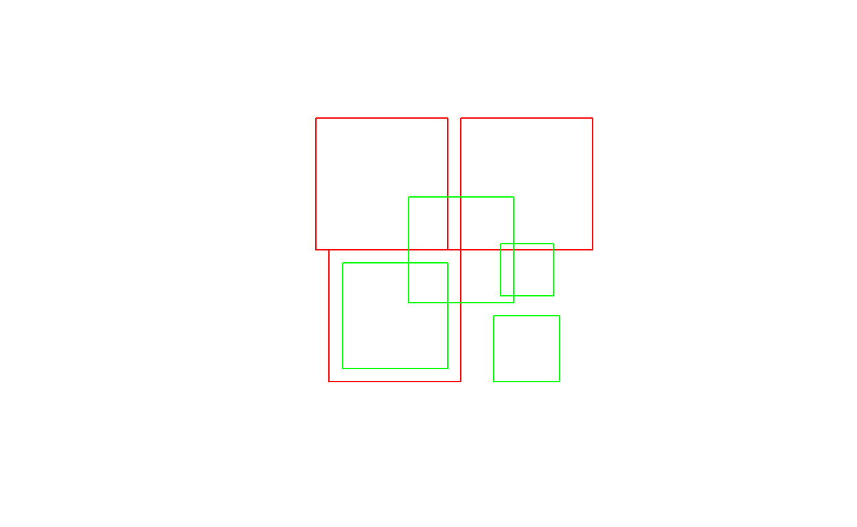
Unary operations
st_is_valid returns whether polygon geometries are topologically valid:
b0 = st_polygon(list(rbind(c(-1,-1), c(1,-1), c(1,1), c(-1,1), c(-1,-1))))
b1 = st_polygon(list(rbind(c(-1,-1), c(1,-1), c(1,1), c(0,-1), c(-1,-1))))
st_is_valid(st_sfc(b0,b1))
[1] TRUE FALSEand st_is_simple whether line geometries are simple:
s = st_sfc(st_linestring(rbind(c(0,0), c(1,1))),
  st_linestring(rbind(c(0,0), c(1,1),c(0,1),c(1,0))))
st_is_simple(s)
[1] TRUE FALSEst_area returns the area of polygon geometries, st_length the
length of line geometries:
st_area(x)[1] 4 4 4[1] 0[1] 2.414214 1.000000st_length(st_sfc(st_multilinestring(list(rbind(c(0,0),c(1,1),c(1,2))),rbind(c(0,0),c(1,0))))) # ignores 2nd part![1] 2.414214Binary operations: distance
st_distance computes the shortest distance matrix between geometries; this is
a dense matrix:
st_distance(x,y) [,1] [,2] [,3] [,4]
[1,] 0.0000000 0.6 0 0.500000
[2,] 0.2828427 0.0 0 1.000000
[3,] 0.2000000 0.8 0 1.220656Binary logical operations:
Binary logical operations return either a sparse matrix
st_intersects(x,y)Sparse geometry binary predicate list of length 3, where the
predicate was `intersects'
1: 1, 3
2: 2, 3
3: 3or a dense matrix
st_intersects(x, x, sparse = FALSE) [,1] [,2] [,3]
[1,] TRUE TRUE TRUE
[2,] TRUE TRUE FALSE
[3,] TRUE FALSE TRUEst_intersects(x, y, sparse = FALSE) [,1] [,2] [,3] [,4]
[1,] TRUE FALSE TRUE FALSE
[2,] FALSE TRUE TRUE FALSE
[3,] FALSE FALSE TRUE FALSEwhere list element i of a sparse matrix contains the indices of
the TRUE elements in row i of the the dense matrix. For large
geometry sets, dense matrices take up a lot of memory and are
mostly filled with FALSE values, hence the default is to return
a sparse matrix.
st_intersects returns for every geometry pair whether they
intersect (dense matrix), or which elements intersect (sparse).
Note that the function st_intersection in this package returns
a geometry for the intersection instead of logicals as in st_intersects (see the next section of this vignette).
Other binary predicates include (using sparse for readability):
st_disjoint(x, y, sparse = FALSE) [,1] [,2] [,3] [,4]
[1,] FALSE TRUE FALSE TRUE
[2,] TRUE FALSE FALSE TRUE
[3,] TRUE TRUE FALSE TRUEst_touches(x, y, sparse = FALSE) [,1] [,2] [,3] [,4]
[1,] FALSE FALSE FALSE FALSE
[2,] FALSE FALSE FALSE FALSE
[3,] FALSE FALSE FALSE FALSEst_crosses(s, s, sparse = FALSE) [,1] [,2]
[1,] FALSE FALSE
[2,] FALSE FALSEst_within(x, y, sparse = FALSE) [,1] [,2] [,3] [,4]
[1,] FALSE FALSE FALSE FALSE
[2,] FALSE FALSE FALSE FALSE
[3,] FALSE FALSE FALSE FALSEst_contains(x, y, sparse = FALSE) [,1] [,2] [,3] [,4]
[1,] TRUE FALSE FALSE FALSE
[2,] FALSE FALSE FALSE FALSE
[3,] FALSE FALSE FALSE FALSEst_overlaps(x, y, sparse = FALSE) [,1] [,2] [,3] [,4]
[1,] FALSE FALSE TRUE FALSE
[2,] FALSE TRUE TRUE FALSE
[3,] FALSE FALSE TRUE FALSEst_equals(x, y, sparse = FALSE) [,1] [,2] [,3] [,4]
[1,] FALSE FALSE FALSE FALSE
[2,] FALSE FALSE FALSE FALSE
[3,] FALSE FALSE FALSE FALSEst_covers(x, y, sparse = FALSE) [,1] [,2] [,3] [,4]
[1,] TRUE FALSE FALSE FALSE
[2,] FALSE FALSE FALSE FALSE
[3,] FALSE FALSE FALSE FALSEst_covered_by(x, y, sparse = FALSE) [,1] [,2] [,3] [,4]
[1,] FALSE FALSE FALSE FALSE
[2,] FALSE FALSE FALSE FALSE
[3,] FALSE FALSE FALSE FALSEst_covered_by(y, y, sparse = FALSE) [,1] [,2] [,3] [,4]
[1,] TRUE FALSE FALSE FALSE
[2,] FALSE TRUE FALSE FALSE
[3,] FALSE FALSE TRUE FALSE
[4,] FALSE FALSE FALSE TRUEst_equals_exact(x, y,0.001, sparse = FALSE) [,1] [,2] [,3] [,4]
[1,] FALSE FALSE FALSE FALSE
[2,] FALSE FALSE FALSE FALSE
[3,] FALSE FALSE FALSE FALSEOperations returning a geometry

par(mfrow=c(1,2), mar = rep(0,4))
plot(st_buffer(u, 0.2))
plot(u, border = 'red', add = TRUE)
plot(st_buffer(u, 0.2), border = 'grey')
plot(u, border = 'red', add = TRUE)
plot(st_buffer(u, -0.2), add = TRUE)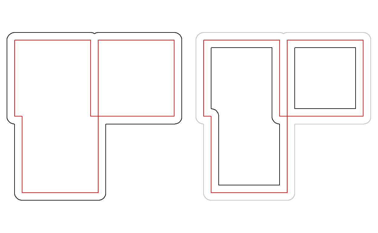
plot(st_boundary(x))
par(mfrow=c(1,2))
plot(x)
plot(st_centroid(x), add = TRUE, col = 'red')
plot(x)
plot(st_centroid(u), add = TRUE, col = 'red')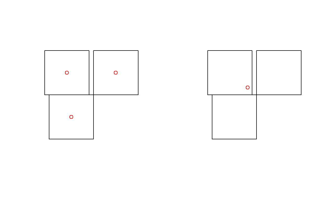
st_intersection:
Note that the function st_intersects returns a logical matrix indicating whether each geometry pair intersects (see the previous section).
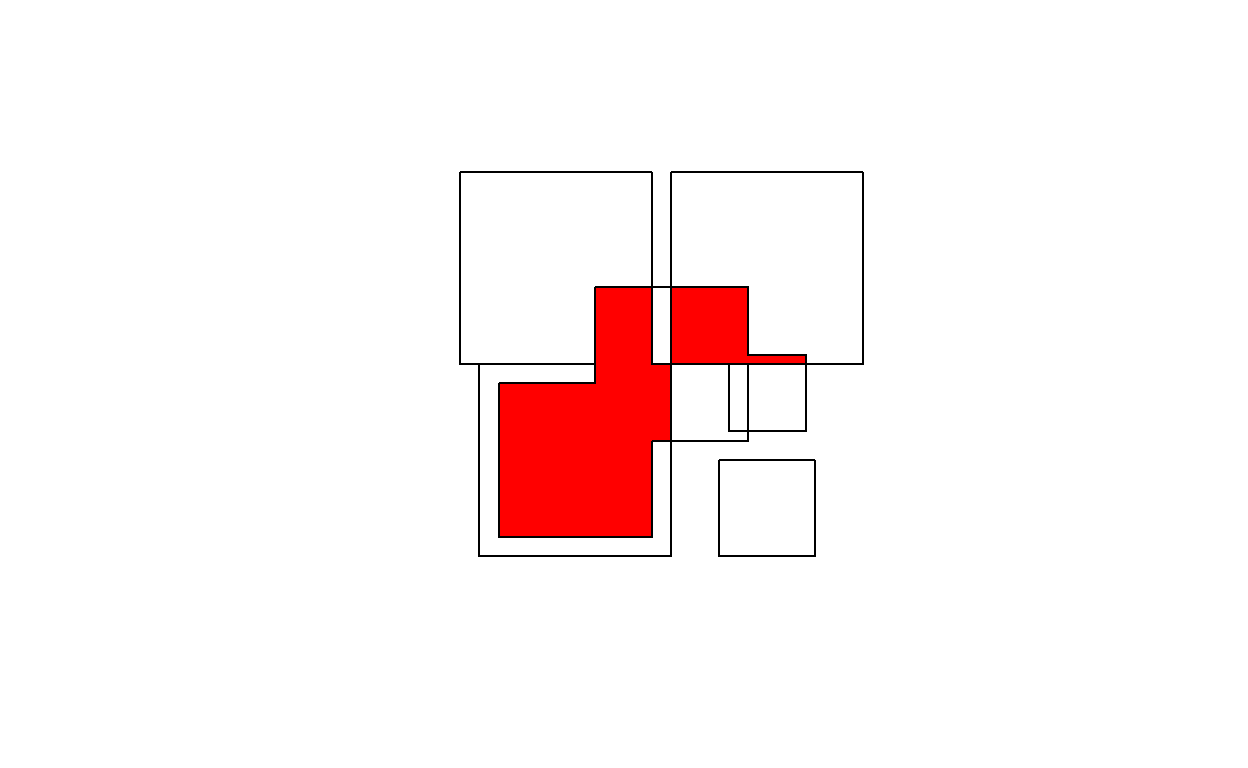
To get everything but the intersection, use st_difference or st_sym_difference:
par(mfrow=c(2,2), mar = c(0,0,1,0))
plot(x, col = '#ff333388');
plot(y, add=TRUE, col='#33ff3388')
title("x: red, y: green")
plot(x, border = 'grey')
plot(st_difference(st_union(x),st_union(y)), col = 'lightblue', add = TRUE)
title("difference(x,y)")
plot(x, border = 'grey')
plot(st_difference(st_union(y),st_union(x)), col = 'lightblue', add = TRUE)
title("difference(y,x)")
plot(x, border = 'grey')
plot(st_sym_difference(st_union(y),st_union(x)), col = 'lightblue', add = TRUE)
title("sym_difference(x,y)")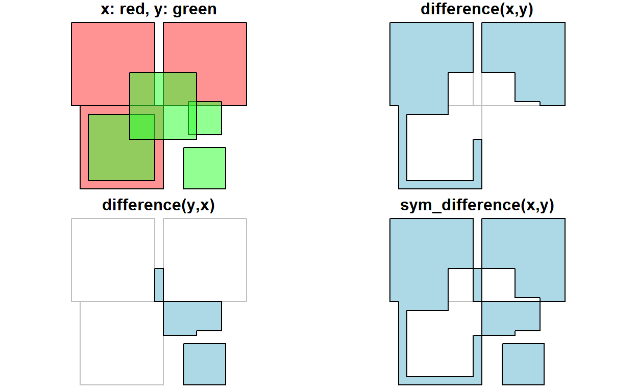
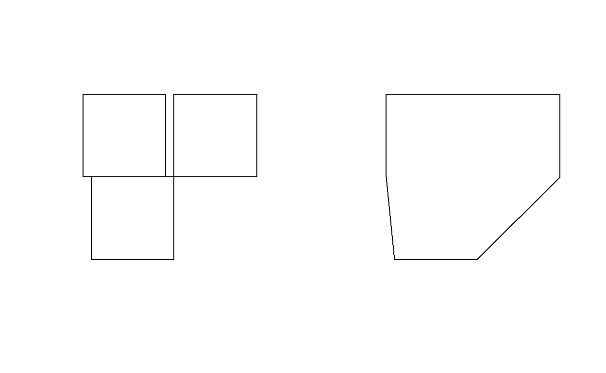
Function st_segmentize adds points to straight line sections of a lines or polygon object:
par(mfrow=c(1,3),mar=c(1,1,0,0))
pts = rbind(c(0,0),c(1,0),c(2,1),c(3,1))
ls = st_linestring(pts)
plot(ls)
points(pts)
ls.seg = st_segmentize(ls, 0.3)
plot(ls.seg)
pts = ls.seg
points(pts)
pol = st_polygon(list(rbind(c(0,0),c(1,0),c(1,1),c(0,1),c(0,0))))
pol.seg = st_segmentize(pol, 0.3)
plot(pol.seg, col = 'grey')
points(pol.seg[[1]])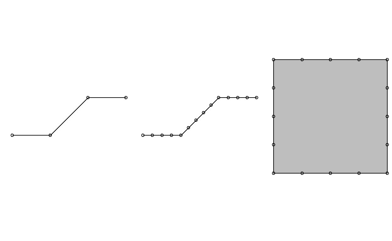
Function st_polygonize polygonizes a multilinestring, as long as the points form a closed polygon:
par(mfrow=c(1,2),mar=c(0,0,1,0))
mls = st_multilinestring(list(matrix(c(0,0,0,1,1,1,0,0),,2,byrow=TRUE)))
x = st_polygonize(mls)
plot(mls, col = 'grey')
title("multilinestring")
plot(x, col = 'grey')
title("polygon")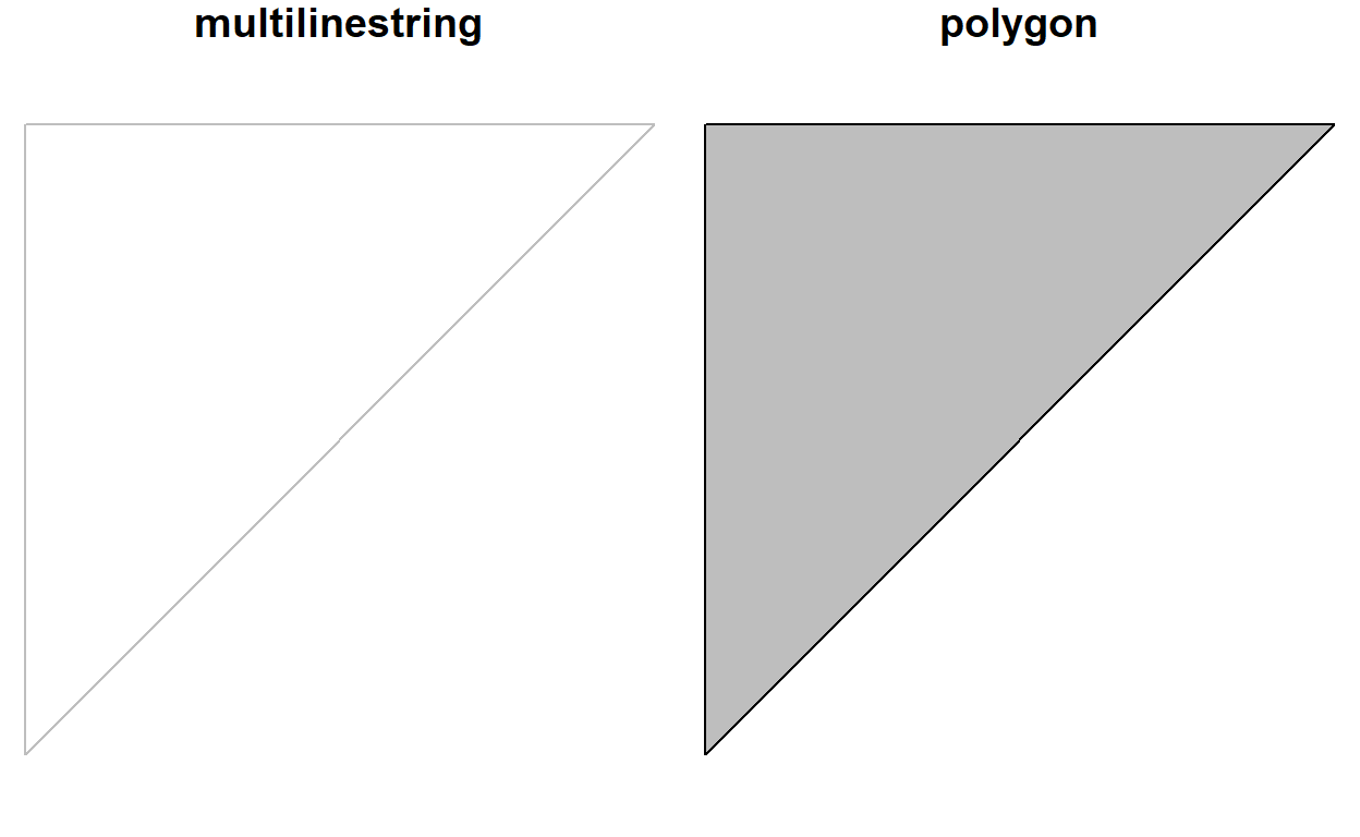
Origin-Destination Data
By request, I am going to show one further example of how to use spatial data in R – origin - destination data analysis. I am going to use data exported from Replica (which you should have access to using your NN email at this link) for people traveling to Downtown Portland from within the City of Portland in Fall 2019. First we will get the the total number of trips totaled by origin and destination TAZ.
pdx_city_boundary = city_bounds_projected %>%
  filter(CITYNAME=="Portland")

#This was too big for GitHub -- has every TAZ in greater NW U.S., so subsetted to just TAZs in Portland.
# full_taz_set = read_sf("data/replica/taz.geojson")
# sub_taz_set = full_taz_set %>%
#   st_transform(coord_local) %>%
#   filter(st_intersects(geometry,pdx_city_boundary,sparse = FALSE)) %>%
#   mutate(whole_area = st_area(geometry) %>% as.numeric()) %>%
#   st_intersection(pdx_city_boundary %>% select(geometry)) %>%
#   mutate(intersect_area = st_area(geometry) %>% as.numeric(),
#          overlap_percent = intersect_area/whole_area) %>%
#   filter(overlap_percent >=0.05)
#
# leaflet() %>%
#   addProviderTiles("CartoDB.Positron") %>%
#   addPolygons(data = sub_taz_set %>% st_transform(4326))
#
# write_rds(sub_taz_set,"data/replica/sub_taz_set.rds")

#Using subset
sub_taz_set = read_rds("data/replica/sub_taz_set.rds")
sub_taz_set
Simple feature collection with 149 features and 6 fields
Geometry type: GEOMETRY
Dimension: XY
Bounding box: xmin: 7604002 ymin: 651321.3 xmax: 7696975 ymax: 732250.2
Projected CRS: NAD83 / Oregon North (ft)
# A tibble: 149 × 7
id label name whole…¹ geometry inter…² overl…³
* <chr> <chr> <chr> <dbl> <GEOMETRY [ft]> <dbl> <dbl>
1 4105… taz 4105… 6.11e7 POLYGON ((7632589 701824… 6.11e7 1.00
2 4105… taz 4105… 1.79e7 POLYGON ((7672015 667639… 1.79e7 1.00
3 4105… taz 4105… 9.92e6 POLYGON ((7656503 699928… 9.92e6 1.00
4 4105… taz 4105… 1.93e7 POLYGON ((7660125 685130… 1.93e7 1.00
5 4105… taz 4105… 1.21e7 MULTIPOLYGON (((7672548 … 7.46e6 0.619
6 4105… taz 4105… 1.21e7 POLYGON ((7655940 677336… 1.21e7 1.00
7 4105… taz 4105… 1.31e7 POLYGON ((7657974 678735… 1.31e7 1
8 4105… taz 4105… 3.04e8 POLYGON ((7610598 709535… 2.95e8 0.970
9 4105… taz 4105… 2.87e7 POLYGON ((7682503 683084… 2.87e7 1.00
10 4105… taz 4105… 2.72e7 POLYGON ((7652163 672158… 2.72e7 1.00
# … with 139 more rows, and abbreviated variable names ¹whole_area,
# ²intersect_area, ³overlap_percentreplica_trips_raw = read_csv("data/replica/replica-places-trips-northwest.zip")
replica_trips_raw# A tibble: 306,276 × 22
activity_id person_id dista…¹ durat…² mode trave…³ previ…⁴ start…⁵
<dbl> <chr> <dbl> <dbl> <chr> <chr> <chr> <chr>
1 4.90e18 30114143… 0 0 WALK… SOCIAL HOME 2019-1…
2 1.52e19 28113985… 161. 60 WALK… EAT HOME 2019-1…
3 8.60e18 88088628… 0 0 WALK… EAT HOME 2019-1…
4 3.10e18 14226367… 0 0 BIKI… EAT HOME 2019-1…
5 5.34e18 14787794… 0 0 WALK… EAT HOME 2019-1…
6 2.90e18 99211811… 0 0 WALK… SOCIAL HOME 2019-1…
7 4.14e18 12595860… 0 0 WALK… EAT HOME 2019-1…
8 7.27e18 12176618… 161. 60 WALK… SHOP HOME 2019-1…
9 8.70e18 11126316… 0 0 WALK… SOCIAL HOME 2019-1…
10 4.68e18 17434900… 0 0 WALK… EAT HOME 2019-1…
# … with 306,266 more rows, 14 more variables:
# start_local_hour <dbl>, end_time <chr>, end_local_hour <dbl>,
# origin_us_taz <chr>, origin_bgrp <chr>, origin_bgrp_lat <dbl>,
# origin_bgrp_lng <dbl>, destination_us_taz <dbl>,
# destination_bgrp <dbl>, destination_bgrp_lat <dbl>,
# destination_bgrp_lng <dbl>, vehicle_type <chr>,
# vehicle_fuel_type <chr>, vehicle_fuel_technology <chr>, and …#sum up origin destination data ourselves
manual_od_summ = replica_trips_raw %>%
group_by(origin_us_taz,destination_us_taz) %>%
summarise(num_trips = n()) %>%
arrange(desc(num_trips))
manual_od_summ# A tibble: 4,884 × 3
# Groups: origin_us_taz [2,251]
origin_us_taz destination_us_taz num_trips
<chr> <dbl> <int>
1 4105100010600 4105100010600 36493
2 4105100005600 4105100005600 24672
3 4105100005100 4105100005100 19932
4 4105100005700 4105100005700 11683
5 4105100010600 4105100005100 3772
6 4105100010600 4105100005600 2920
7 4105100005100 4105100010600 2600
8 4105100005600 4105100010600 2500
9 4105100005700 4105100005600 2353
10 4105100005600 4105100005700 2006
# … with 4,874 more rows#Or use Replica's shortcut output
replica_od_raw = read_csv("data/replica/od_thursday_sep2019-nov2019_northwest_4filters_created12-08-2021.zip")
replica_od_raw# A tibble: 4,884 × 31
origin_name desti…¹ total…² age_u…³ age_5…⁴ age_1…⁵ age_1…⁶ age_3…⁷
<chr> <dbl> <dbl> <dbl> <dbl> <dbl> <dbl> <dbl>
1 5306700000… 4.11e12 1 0 0 0 0 1
2 4105100009… 4.11e12 118 0 0 0 29 45
3 4100500022… 4.11e12 35 0 0 0 3 10
4 4105100004… 4.11e12 271 0 1 1 75 45
5 4101700001… 4.11e12 2 0 0 0 1 1
6 4106700030… 4.11e12 19 0 0 0 2 4
7 1605700LT6… 4.11e12 1 0 0 0 1 0
8 4100500022… 4.11e12 43 0 0 0 6 22
9 5301100041… 4.11e12 5 0 0 0 1 0
10 4104100950… 4.11e12 16 0 0 0 2 0
# … with 4,874 more rows, 23 more variables: age_50_to_64 <dbl>,
# age_over_65 <dbl>, age_visitor <dbl>,
# race_hispanic_or_latino_origin <dbl>,
# race_black_not_hispanic_or_latino <dbl>,
# race_white_not_hispanic_or_latino <dbl>,
# race_asian_not_hispanic_or_latino <dbl>,
# race_two_races_not_hispanic_or_latino <dbl>, …shortcut_od_summ = replica_od_raw %>%
rename(origin_us_taz = origin_name,
destination_us_taz = destination_name) %>%
group_by(origin_us_taz,destination_us_taz) %>%
summarise(num_trips = sum(total_count)) %>%
arrange(desc(num_trips))
shortcut_od_summ# A tibble: 4,884 × 3
# Groups: origin_us_taz [2,251]
origin_us_taz destination_us_taz num_trips
<chr> <dbl> <dbl>
1 4105100010600 4105100010600 36493
2 4105100005600 4105100005600 24672
3 4105100005100 4105100005100 19932
4 4105100005700 4105100005700 11683
5 4105100010600 4105100005100 3772
6 4105100010600 4105100005600 2920
7 4105100005100 4105100010600 2600
8 4105100005600 4105100010600 2500
9 4105100005700 4105100005600 2353
10 4105100005600 4105100005700 2006
# … with 4,874 more rows#I prefer the manual route, we'll continue with that to the next stepSee the stplanr package and its od2line() function (and a webinar in which Ulises demonstrated this) for a shortcut, but we can build our OD lines manually from the above understanding of sf geometries! We just need centroids, and then to construct straight lines between them.
I did only compute these flows in one direction, since the Replica query was only for trips with destinations in Downtown Portland. Often, you will want to use bi-directional flows; I will develop a copy-paste script for this in 2022, but for now please look at the webinar referred to above where Ulises demonstrated how to do this.
I have commented the script below with step-by-step descriptions, and will talk through it verbally in the webinar (a recording of which is available above).
library(scales)

taz_centroids = sub_taz_set %>%
  #convert polygons to centroids (points)
  st_centroid() %>%
  #Get rid of unneccesary columns
  select(-contains("area"),-contains("percent"))
# Have a look a the centroids
taz_centroids
Simple feature collection with 149 features and 3 fields
Geometry type: POINT
Dimension: XY
Bounding box: xmin: 7619339 ymin: 654082.2 xmax: 7693632 ymax: 716758.3
Projected CRS: NAD83 / Oregon North (ft)
# A tibble: 149 × 4
id label name geometry
<chr> <chr> <chr> <POINT [ft]>
1 4105100980000 taz 4105100980000 (7637138 698140.2)
2 4105100000602 taz 4105100000602 (7670668 666001.7)
3 4105100003603 taz 4105100003603 (7657866 700288.7)
4 4105100001900 taz 4105100001900 (7657833 685205.3)
5 4105100007800 taz 4105100007800 (7673642 693175.8)
6 4105100000901 taz 4105100000901 (7655780 675948.7)
7 4105100001400 taz 4105100001400 (7659302 679674.9)
8 4105100004300 taz 4105100004300 (7621410 705033.1)
9 4105100009201 taz 4105100009201 (7681946 679759.4)
10 4105100001000 taz 4105100001000 (7650957 674966.6)
# … with 139 more rowsuq_lines_in_replica = manual_od_summ %>%
#Create an identifier for the OD lines we are going to construct
mutate(od_line_id = paste0(origin_us_taz,"-",destination_us_taz)) %>%
#Get unique line IDs
distinct(od_line_id)
od_lines = expand_grid( # create 'expanded' data frame of all unique combinations
origin_us_taz = taz_centroids$id,
destination_us_taz = taz_centroids$id
) %>%
#Use identifier to filter for flows only within the Replica dataset (i.e. removing OD pairs from outside Portland and not destinating downtown)
mutate(od_line_id = paste0(origin_us_taz,"-",destination_us_taz)) %>%
filter(od_line_id %in% uq_lines_in_replica$od_line_id) %>%
# Construct geometry using an anonymous function (i.e. defined on the fly), iterating with purrr
mutate(geometry = pmap(.l = list(origin_us_taz, destination_us_taz),
.f = function(otaz,dtaz){
# for debugging only
# x=1
# otaz = od_lines$origin_us_taz[x]
# dtaz = od_lines$destination_us_taz[x]
#create matrix of two coordinate points
points = rbind(
taz_centroids %>% filter(id == otaz) %>% st_coordinates(),
taz_centroids %>% filter(id == dtaz) %>% st_coordinates()
)
#create linestring from matrix
line = st_linestring(points)
#return linestring
return(line)
}) %>%
#Convert to SF column, assign CRS
st_sfc(crs = coord_local)) %>%
#Coerce tbl into sf data frame
st_as_sf()
#Used for leaflet map - TAZs of Downtown Portland
destination_tazs = c('4105100005700','4105100010600','4105100005600','4105100005100')
#Joining in the trip sums from replica
od_lines_joined = od_lines %>%
left_join(manual_od_summ %>%
mutate(origin_us_taz = as.character(origin_us_taz),
destination_us_taz = as.character(destination_us_taz))) %>%
#Arrange descending in terms of number of trips
arrange(desc(num_trips)) %>%
#Transform to WGS84 for mapping
st_transform(coord_global) %>%
#Remove internal trips (within a single zone)
filter(origin_us_taz != destination_us_taz)
#Leaflet map
leaflet() %>%
addProviderTiles("CartoDB.Positron") %>%
addPolylines(data = od_lines_joined, weight=~num_trips*0.01,
group =~ destination_us_taz,
label=~ paste0(origin_us_taz," to ",destination_us_taz,": ",
comma(num_trips,accuracy = 1)," weekday daily trips")) %>%
addLayersControl(baseGroups = destination_tazs,
options = layersControlOptions(collapsed = FALSE)) Area-Weighted Aggregation
Let’s say I wanted to find the total estimate of trips (from the Replica dataset) terminating within 1/2 mile of the Nelson\Nygaard office. This is a nonsensical example, but is a simple demonstration of using the st_interpolate_aw function for area-weighted aggregation. Here I use it within a map_*() function so that it can be applied within a series of pipes (%>%).
Note the extensive parameter – from the documentation: logical; if TRUE, the attribute variables are assumed to be spatially extensive (like population) and the sum is preserved, otherwise, spatially intensive (like population density) and the mean is preserved.
nn_buffer = st_point(c(-122.6790507879488,45.519333157798975)) %>%
  st_sfc(crs=4326) %>%
  as_tibble_col("geometry") %>%
  st_as_sf() %>%
  st_transform(coord_local) %>%
  st_buffer(5280/2)

nn_buffer
Simple feature collection with 1 feature and 0 fields
Geometry type: POLYGON
Dimension: XY
Bounding box: xmin: 7641006 ymin: 680327.5 xmax: 7646286 ymax: 685607.5
Projected CRS: NAD83 / Oregon North (ft)
# A tibble: 1 × 1
geometry
* <POLYGON [ft]>
1 ((7646286 682967.5, 7646282 682829.3, 7646272 682691.6, 7646254 682…replica_dest_summ = manual_od_summ %>%
group_by(destination_us_taz) %>%
summarise(num_trips = sum(num_trips)) %>%
mutate(destination_us_taz = as.character(destination_us_taz)) %>%
left_join(sub_taz_set %>%
select(id,geometry) %>%
rename(destination_us_taz = id)) %>%
st_as_sf() %>%
st_transform(coord_local)
replica_dest_summSimple feature collection with 4 features and 2 fields
Geometry type: POLYGON
Dimension: XY
Bounding box: xmin: 7641047 ymin: 675896.7 xmax: 7647056 ymax: 689752.1
Projected CRS: NAD83 / Oregon North (ft)
# A tibble: 4 × 3
destination_us_taz num_trips geometry
* <chr> <int> <POLYGON [ft]>
1 4105100005100 59982 ((7642640 686646.4, 7642638 686910.9, …
2 4105100005600 71362 ((7641486 679549.1, 7641444 679600.2, …
3 4105100005700 42245 ((7644697 676063.4, 7644671 676062.7, …
4 4105100010600 132687 ((7643164 681427.8, 7642904 681534.3, …#So you can compare the two visually
leaflet() %>%
addProviderTiles('CartoDB.Positron') %>%
addPolygons(data = replica_dest_summ %>% st_transform(coord_global),
weight=2,fillOpacity = 0.5,opacity=1,color="white",
fillColor = "blue", label=~destination_us_taz) %>%
addPolygons(data = nn_buffer %>% st_transform(coord_global),
weight=2, fillOpacity = 0.5,opacity = 1,color="white",
fillColor = "red", label= "NN 1/2 mile buffer")nn_buff_with_trips = nn_buffer %>%
mutate(half_mile_trips = map_dbl(.,~st_interpolate_aw(replica_dest_summ %>%
select(num_trips,geometry),
.x,extensive = TRUE) %>%
st_drop_geometry() %>%
pull(num_trips)))
nn_buff_with_tripsSimple feature collection with 1 feature and 1 field
Geometry type: POLYGON
Dimension: XY
Bounding box: xmin: 7641006 ymin: 680327.5 xmax: 7646286 ymax: 685607.5
Projected CRS: NAD83 / Oregon North (ft)
# A tibble: 1 × 2
geometry half_…¹
* <POLYGON [ft]> <dbl>
1 ((7646286 682967.5, 7646282 682829.3, 7646272 682691.6, 764… 163532.
# … with abbreviated variable name ¹half_mile_tripsReference Materials
Further Reading
- Geocomputation with R (web version)
- Applied Spatial Data Analysis with R (PDF version)
- An Introduction to R for Spatial Analysis and Mapping (available where books are sold)
Cheat Sheets
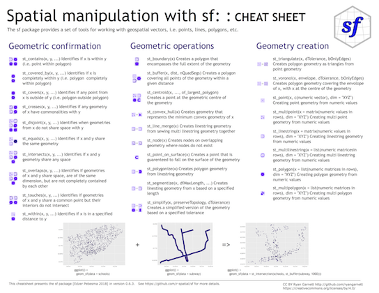
Simple Features (sf) Cheat Sheet
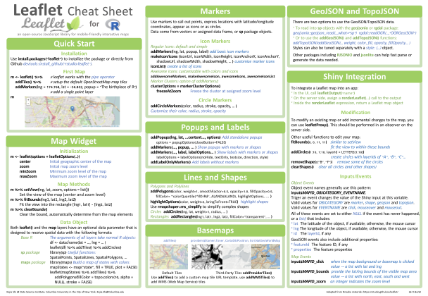
Leaflet for R Cheat Sheet
Related DataCamp Courses
- Spatial data with R (4 courses, 16 hours, includes leaflet course noted below)
- Interactive Maps with leaflet (1 course, 4 hours)
This content was presented to Nelson\Nygaard Staff at a Lunch and Learn webinar on Thursday, December 9th, 2021, and is available as a recording here and embedded above.