This content was presented to Nelson\Nygaard Staff at a Lunch and Learn webinar on Friday, September 4th, 2020, and is available as a recording here and embedded below
Introduction
There are several reasons why learning to use the geospatial capabilities of R are invaluable for R users, especially at Nelson\Nygaard:
- Open source - no ESRI licenses neccessary: R is a completely open source programming language, and so there are not licenses necessary to access its geospatial packages. NN as a firm has a limited number of licenses available at any given time, and the ongoing telecommuting associated with the COVID-19 pandemic has made using GIS licenses more difficult. R can allow you to conduct geospatial analyses on your local machine with no need for licenses.
- Combining spatial and aspatial analyses: As transportation planners, most of the work we do has some spatial component. Because of that, analysis is often separated into GIS and Excel components. With R, that separation is unneccesary – you can combine spatial and aspatial analysis procedures and data seamlessly.
- Automation and processing speed: Like with all other R based analyses, you can automate analysis procedures you have to conduct many times over, potentially speeding up some GIS workflows that are repetitive.
- Modular: Additionally, if written appropriately, commonly conducted analysis procedures can be abstracted into modular code that can be applied across different projects, saving time as a firm.
- Interactive: Because of
leaflet, which we will discuss below, R offers a very low barrier to quickly producing interactive maps, which are both helpful for data exploration and for presentation, especially as increasingly more deliverables move to digital formats.
This module will discuss the spatial data package sf, which is well integrated into the tidyverse and other mapping related packages (including leaflet). There are other spatial data frameworks that came before sf that will not be discussed below (like sp) but are still relevant to understand at a basic level. Reference articles are included below. Additionally, this module will discuss leaflet, an interactive mapping framework that lends itself well to spatial analysis and visualization in R.
Simple Features
Acknowledgment: This portion of this module heavily draws upon, including direct copy-paste of markdown content, the vignettes developed for the sf package, available on the package documentation website.
Simple features or simple feature access refers to a formal standard (ISO 19125-1:2004) that describes how objects in the real world can be represented in computers, with emphasis on the spatial geometry of these objects. It also describes how such objects can be stored in and retrieved from databases, and which geometrical operations should be defined for them.
The standard is widely implemented in spatial databases (such as PostGIS), commercial GIS (e.g., ESRI ArcGIS) and forms the vector data basis for libraries such as GDAL. A subset of simple features forms the GeoJSON standard.
R has well-supported classes for storing spatial data (sp) and interfacing to the above mentioned environments (rgdal, rgeos), but has so far lacked a complete implementation of simple features, making conversions at times convoluted, inefficient or incomplete. The package sf tries to fill this gap, and aims at succeeding sp in the long term.
This vignette:
- explains what is meant by features, and by simple features
- shows how they are implemented in R
- provides examples of how you can work with them
- shows how they can be read from and written to external files or resources
- discusses how they can be converted to and from sp objects
- shows how they can be used for meaningful spatial analysis
What is a feature?
A feature is thought of as a thing, or an object in the real world, such as a building or a tree. As is the case with objects, they often consist of other objects. This is the case with features too: a set of features can form a single feature. A forest stand can be a feature, a forest can be a feature, a city can be a feature. A satellite image pixel can be a feature, a complete image can be a feature too.
Features have a geometry describing where on Earth the feature is located, and they have attributes, which describe other properties. The geometry of a tree can be the delineation of its crown, of its stem, or the point indicating its centre. Other properties may include its height, color, diameter at breast height at a particular date, and so on.
The standard says: “A simple feature is defined by the OpenGIS Abstract specification to have both spatial and non-spatial attributes. Spatial attributes are geometry valued, and simple features are based on 2D geometry with linear interpolation between vertices.” We will see soon that the same standard will extend its coverage beyond 2D and beyond linear interpolation. Here, we take simple features as the data structures and operations described in the standard.
Dimensions
All geometries are composed of points. Points are coordinates in a 2-, 3- or 4-dimensional space. All points in a geometry have the same dimensionality. In addition to X and Y coordinates, there are two optional additional dimensions:
- a Z coordinate, denoting altitude
- an M coordinate (rarely used), denoting some measure that is associated with the point, rather than with the feature as a whole (in which case it would be a feature attribute); examples could be time of measurement, or measurement error of the coordinates
The four possible cases then are:
- two-dimensional points refer to x and y, easting and northing, or longitude and latitude, we refer to them as XY
- three-dimensional points as XYZ
- three-dimensional points as XYM
- four-dimensional points as XYZM (the third axis is Z, fourth M)
Simple feature geometry types
The following seven simple feature types are the most common, and are for instance the only ones used for GeoJSON:
| type | description |
|---|---|
POINT |
zero-dimensional geometry containing a single point |
LINESTRING |
sequence of points connected by straight, non-self intersecting line pieces; one-dimensional geometry |
POLYGON |
geometry with a positive area (two-dimensional); sequence of points form a closed, non-self intersecting ring; the first ring denotes the exterior ring, zero or more subsequent rings denote holes in this exterior ring |
MULTIPOINT |
set of points; a MULTIPOINT is simple if no two Points in the MULTIPOINT are equal |
MULTILINESTRING |
set of linestrings |
MULTIPOLYGON |
set of polygons |
GEOMETRYCOLLECTION |
set of geometries of any type except GEOMETRYCOLLECTION |
Each of the geometry types can also be a (typed) empty set, containing zero coordinates (for POINT the standard is not clear how to represent the empty geometry). Empty geometries can be thought of being the analogue to missing (NA) attributes, NULL values or empty lists.
The remaining geometries 10 are rarer, but increasingly find implementations:
| type | description |
|---|---|
CIRCULARSTRING |
The CIRCULARSTRING is the basic curve type, similar to a LINESTRING in the linear world. A single segment requires three points, the start and end points (first and third) and any other point on the arc. The exception to this is for a closed circle, where the start and end points are the same. In this case the second point MUST be the center of the arc, i.e., the opposite side of the circle. To chain arcs together, the last point of the previous arc becomes the first point of the next arc, just like in LINESTRING. This means that a valid circular string must have an odd number of points greater than 1. |
COMPOUNDCURVE |
A compound curve is a single, continuous curve that has both curved (circular) segments and linear segments. That means that in addition to having well-formed components, the end point of every component (except the last) must be coincident with the start point of the following component. |
CURVEPOLYGON |
Example compound curve in a curve polygon: CURVEPOLYGON(COMPOUNDCURVE(CIRCULARSTRING(0 0,2 0, 2 1, 2 3, 4 3),(4 3, 4 5, 1 4, 0 0)), CIRCULARSTRING(1.7 1, 1.4 0.4, 1.6 0.4, 1.6 0.5, 1.7 1) ) |
MULTICURVE |
A MultiCurve is a 1-dimensional GeometryCollection whose elements are Curves, it can include linear strings, circular strings or compound strings. |
MULTISURFACE |
A MultiSurface is a 2-dimensional GeometryCollection whose elements are Surfaces, all using coordinates from the same coordinate reference system. |
CURVE |
A Curve is a 1-dimensional geometric object usually stored as a sequence of Points, with the subtype of Curve specifying the form of the interpolation between Points |
SURFACE |
A Surface is a 2-dimensional geometric object |
POLYHEDRALSURFACE |
A PolyhedralSurface is a contiguous collection of polygons, which share common boundary segments |
TIN |
A TIN (triangulated irregular network) is a PolyhedralSurface consisting only of Triangle patches. |
TRIANGLE |
A Triangle is a polygon with 3 distinct, non-collinear vertices and no interior boundary |
Note that CIRCULASTRING, COMPOUNDCURVE and CURVEPOLYGON are not described in the SFA standard, but in the SQL-MM part 3 standard. The descriptions above were copied from the PostGIS manual.
Coordinate reference system
Coordinates can only be placed on the Earth’s surface when their coordinate reference system (CRS) is known; this may be a spheroid CRS such as WGS84, a projected, two-dimensional (Cartesian) CRS such as a UTM zone or Web Mercator, or a CRS in three-dimensions, or including time. Similarly, M-coordinates need an attribute reference system, e.g. a measurement unit.
How simple features in R are organized
Package sf represents simple features as native R objects. Similar to PostGIS, all functions and methods in sf that operate on spatial data are prefixed by st_, which refers to spatial type; this makes them easily findable by command-line completion. Simple features are implemented as R native data, using simple data structures (S3 classes, lists, matrix, vector). Typical use involves reading, manipulating and writing of sets of features, with attributes and geometries.
As attributes are typically stored in data.frame objects (or the very similar tbl_df), we will also store feature geometries in a data.frame column. Since geometries are not single-valued, they are put in a list-column, a list of length equal to the number of records in the data.frame, with each list element holding the simple feature geometry of that feature. The three classes used to represent simple features are:
sf, the table (data.frame) with feature attributes and feature geometries, which containssfc, the list-column with the geometries for each feature (record), which is composed ofsfg, the feature geometry of an individual simple feature.
We will now discuss each of these three classes.
sf: objects with simple features
As we usually do not work with geometries of single simple features, but with datasets consisting of sets of features with attributes, the two are put together in sf (simple feature) objects. The following command reads the nc dataset from a file that is contained in the sf package:
library(sf)
nc <- st_read(system.file("shape/nc.shp", package="sf"))
Reading layer `nc' from data source `C:\Users\blancb\Local\R\win-library\4.0\sf\shape\nc.shp' using driver `ESRI Shapefile'
Simple feature collection with 100 features and 14 fields
geometry type:  MULTIPOLYGON
dimension:      XY
bbox:           xmin: -84.32385 ymin: 33.88199 xmax: -75.45698 ymax: 36.58965
geographic CRS: NAD27
(Note that users will not use system.file but give a filename directly, and that shapefiles consist of more than one file, all with identical basename, which reside in the same directory.) The short report printed gives the file name, the driver (ESRI Shapefile), mentions that there are 100 features (records, represented as rows) and 14 fields (attributes, represented as columns). This object is of class
class(nc)
[1] "sf" "data.frame"meaning it extends (and “is” a) data.frame, but with a single list-column with geometries, which is held in the column with name
attr(nc, "sf_column")
[1] "geometry"If we print the first three features, we see their attribute values and an abridged version of the geometry
print(nc[9:15], n = 3)
which would give the following output:
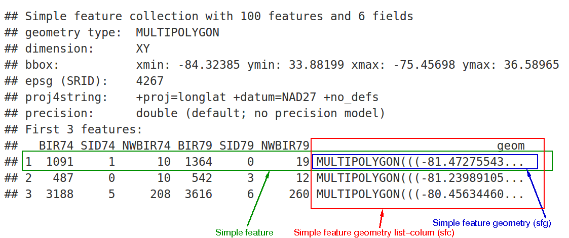
In the output we see:
- in green a simple feature: a single record, or
data.framerow, consisting of attributes and geometry - in blue a single simple feature geometry (an object of class
sfg) - in red a simple feature list-column (an object of class
sfc, which is a column in thedata.frame) - that although geometries are native R objects, they are printed as well-known text
sf objects are
methods(class = "sf")
 [1] $<-                   [                     [[<-
 [4] aggregate             anti_join             arrange
 [7] as.data.frame         cbind                 clean_names
[10] coerce                dbDataType            dbWriteTable
[13] distinct              dplyr_reconstruct     filter
[16] full_join             gather                group_by
[19] group_split           identify              initialize
[22] inner_join            left_join             merge
[25] mutate                nest                  plot
[28] print                 rbind                 rename
[31] right_join            sample_frac           sample_n
[34] select                semi_join             separate
[37] separate_rows         show                  slice
[40] slotsFromS3           spread                st_agr
[43] st_agr<-              st_area               st_as_s2
[46] st_as_sf              st_bbox               st_boundary
[49] st_buffer             st_cast               st_centroid
[52] st_collection_extract st_convex_hull        st_coordinates
[55] st_crop               st_crs                st_crs<-
[58] st_difference         st_filter             st_geometry
[61] st_geometry<-         st_interpolate_aw     st_intersection
[64] st_intersects         st_is                 st_is_valid
[67] st_join               st_line_merge         st_m_range
[70] st_make_valid         st_nearest_points     st_node
[73] st_normalize          st_point_on_surface   st_polygonize
[76] st_precision          st_reverse            st_sample
[79] st_segmentize         st_set_precision      st_shift_longitude
[82] st_simplify           st_snap               st_sym_difference
[85] st_transform          st_triangulate        st_union
[88] st_voronoi            st_wrap_dateline      st_write
[91] st_z_range            st_zm                 summarise
[94] transform             transmute             ungroup
[97] unite                 unnest
see '?methods' for accessing help and source codedata.frame objects with geometry list-columns that are not of class sf, e.g. by
nc.no_sf <- as.data.frame(nc)
class(nc.no_sf)
[1] "data.frame"However, such objects:
- no longer register which column is the geometry list-column
- no longer have a plot method, and
- lack all of the other dedicated methods listed above for class
sf
sfc: simple feature geometry list-column
The column in the sf data.frame that contains the geometries is a list, of class sfc. We can retrieve the geometry list-column in this case by nc$geom or nc[[15]], but the more general way uses st_geometry:
(nc_geom <- st_geometry(nc))
Geometry set for 100 features
geometry type:  MULTIPOLYGON
dimension:      XY
bbox:           xmin: -84.32385 ymin: 33.88199 xmax: -75.45698 ymax: 36.58965
geographic CRS: NAD27
First 5 geometries:
Geometries are printed in abbreviated form, but we can can view a complete geometry by selecting it, e.g. the first one by
nc_geom[[1]]
The way this is printed is called well-known text, and is part of the standards. The word MULTIPOLYGON is followed by three parenthesis, because it can consist of multiple polygons, in the form of MULTIPOLYGON(POL1,POL2), where POL1 might consist of an exterior ring and zero or more interior rings, as of (EXT1,HOLE1,HOLE2). Sets of coordinates are held together with parenthesis, so we get ((crds_ext)(crds_hole1)(crds_hole2)) where crds_ is a comma-separated set of coordinates of a ring. This leads to the case above, where MULTIPOLYGON(((crds_ext))) refers to the exterior ring (1), without holes (2), of the first polygon (3) - hence three parentheses.
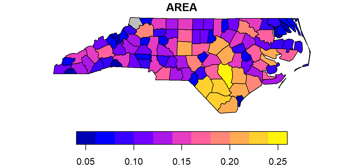
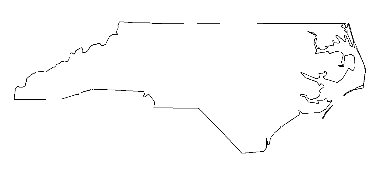
We can see there is a single polygon with no rings:
par(mar = c(0,0,1,0))
plot(nc[1], reset = FALSE) # reset = FALSE: we want to add to a plot with a legend
plot(nc[1,1], col = 'grey', add = TRUE)
Following the MULTIPOLYGON datastructure, in R we have a list of lists of lists of matrices. For instance, we get the first 3 coordinate pairs of the second exterior ring (first ring is always exterior) for the geometry of feature 4 by
nc_geom[[4]][[2]][[1]][1:3,]
          [,1]     [,2]
[1,] -76.02717 36.55672
[2,] -75.99866 36.55665
[3,] -75.91192 36.54253
Geometry columns have their own class,
class(nc_geom)
[1] "sfc_MULTIPOLYGON" "sfc" methods(class = 'sfc')
 [1] [                     [<-                   as.data.frame
 [4] c                     coerce                format
 [7] fortify               identify              initialize
[10] obj_sum               Ops                   print
[13] rep                   scale_type            show
[16] slotsFromS3           st_area               st_as_binary
[19] st_as_grob            st_as_s2              st_as_sf
[22] st_as_text            st_bbox               st_boundary
[25] st_buffer             st_cast               st_centroid
[28] st_collection_extract st_convex_hull        st_coordinates
[31] st_crop               st_crs                st_crs<-
[34] st_difference         st_geometry           st_intersection
[37] st_intersects         st_is                 st_is_valid
[40] st_line_merge         st_m_range            st_make_valid
[43] st_nearest_points     st_node               st_normalize
[46] st_point_on_surface   st_polygonize         st_precision
[49] st_reverse            st_sample             st_segmentize
[52] st_set_precision      st_shift_longitude    st_simplify
[55] st_snap               st_sym_difference     st_transform
[58] st_triangulate        st_union              st_voronoi
[61] st_wrap_dateline      st_write              st_z_range
[64] st_zm                 str                   summary
[67] type_sum              vec_cast.sfc          vec_ptype2.sfc
see '?methods' for accessing help and source code
Coordinate reference systems (st_crs and st_transform) are discussed in the section on coordinate reference systems. st_as_wkb and st_as_text convert geometry list-columns into well-known-binary or well-known-text, explained below. st_bbox retrieves the coordinate bounding box.
attributes(nc_geom)
$n_empty
[1] 0

$crs
Coordinate Reference System:
  User input: NAD27
  wkt:
GEOGCRS["NAD27",
    DATUM["North American Datum 1927",
        ELLIPSOID["Clarke 1866",6378206.4,294.978698213898,
            LENGTHUNIT["metre",1]]],
    PRIMEM["Greenwich",0,
        ANGLEUNIT["degree",0.0174532925199433]],
    CS[ellipsoidal,2],
        AXIS["latitude",north,
            ORDER[1],
            ANGLEUNIT["degree",0.0174532925199433]],
        AXIS["longitude",east,
            ORDER[2],
            ANGLEUNIT["degree",0.0174532925199433]],
    ID["EPSG",4267]]

$class
[1] "sfc_MULTIPOLYGON" "sfc"

$precision
[1] 0

$bbox
     xmin      ymin      xmax      ymax
-84.32385  33.88199 -75.45698  36.58965
Mixed geometry types
The class of nc_geom is c("sfc_MULTIPOLYGON", "sfc"): sfc is shared with all geometry types, and sfc_TYPE with TYPE indicating the type of the particular geometry at hand.
GEOMETRYCOLLECTION, and GEOMETRY. GEOMETRYCOLLECTION indicates that each of the geometries may contain a mix of geometry types, as in
(mix <- st_sfc(st_geometrycollection(list(st_point(1:2))),
    st_geometrycollection(list(st_linestring(matrix(1:4,2))))))
Geometry set for 2 features
geometry type:  GEOMETRYCOLLECTION
dimension:      XY
bbox:           xmin: 1 ymin: 2 xmax: 2 ymax: 4
CRS: NAclass(mix)
[1] "sfc_GEOMETRYCOLLECTION" "sfc" Still, the geometries are here of a single type.
The secondGEOMETRY, indicates that the geometries in the geometry list-column are of varying type:
(mix <- st_sfc(st_point(1:2), st_linestring(matrix(1:4,2))))
Geometry set for 2 features
geometry type:  GEOMETRY
dimension:      XY
bbox:           xmin: 1 ymin: 2 xmax: 2 ymax: 4
CRS: NAclass(mix)
[1] "sfc_GEOMETRY" "sfc" These two are fundamentally different: GEOMETRY is a superclass without instances, GEOMETRYCOLLECTION is a geometry instance. GEOMETRY list-columns occur when we read in a data source with a mix of geometry types. GEOMETRYCOLLECTION is a single feature’s geometry: the intersection of two feature polygons may consist of points, lines and polygons, see the example below.
sfg: simple feature geometry
Simple feature geometry (sfg) objects carry the geometry for a single feature, e.g. a point, linestring or polygon.
Simple feature geometries are implemented as R native data, using the following rules
- a single POINT is a numeric vector
- a set of points, e.g. in a LINESTRING or ring of a POLYGON is a
matrix, each row containing a point - any other set is a
list
Creator functions are rarely used in practice, since we typically bulk read and write spatial data. They are useful for illustration:
'XY' num [1:2] 1 2 'XYZ' num [1:3] 1 2 3 'XYM' num [1:3] 1 2 3 'XYZM' num [1:4] 1 2 3 4st_zm(x, drop = TRUE, what = "ZM")
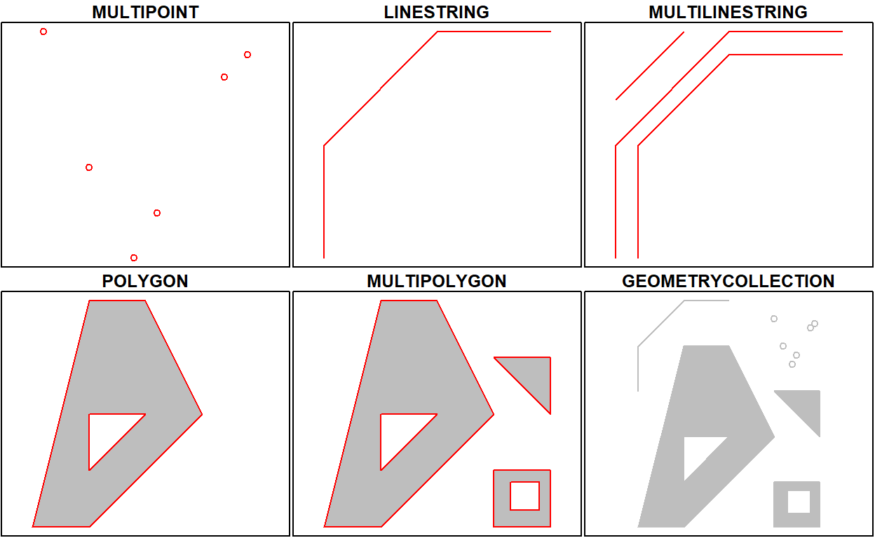
This means that we can represent 2-, 3- or 4-dimensional coordinates. All geometry objects inherit from sfg (simple feature geometry), but also have a type (e.g. POINT), and a dimension (e.g. XYM) class name. A figure illustrates six of the seven most common types.
With the exception of the POINT which has a single point as geometry, the remaining six common single simple feature geometry types that correspond to single features (single records, or rows in a data.frame) are created like this
p <- rbind(c(3.2,4), c(3,4.6), c(3.8,4.4), c(3.5,3.8), c(3.4,3.6), c(3.9,4.5))
(mp <- st_multipoint(p))
s1 <- rbind(c(0,3),c(0,4),c(1,5),c(2,5))
(ls <- st_linestring(s1))
s2 <- rbind(c(0.2,3), c(0.2,4), c(1,4.8), c(2,4.8))
s3 <- rbind(c(0,4.4), c(0.6,5))
(mls <- st_multilinestring(list(s1,s2,s3)))
p1 <- rbind(c(0,0), c(1,0), c(3,2), c(2,4), c(1,4), c(0,0))
p2 <- rbind(c(1,1), c(1,2), c(2,2), c(1,1))
pol <-st_polygon(list(p1,p2))
p3 <- rbind(c(3,0), c(4,0), c(4,1), c(3,1), c(3,0))
p4 <- rbind(c(3.3,0.3), c(3.8,0.3), c(3.8,0.8), c(3.3,0.8), c(3.3,0.3))[5:1,]
p5 <- rbind(c(3,3), c(4,2), c(4,3), c(3,3))
(mpol <- st_multipolygon(list(list(p1,p2), list(p3,p4), list(p5))))
(gc <- st_geometrycollection(list(mp, mpol, ls)))
The objects created are shown here:
Geometries can also be empty, as in
(x <- st_geometrycollection())
length(x)
[1] 0Well-known text, well-known binary, precision
WKT and WKB
Well-known text (WKT) and well-known binary (WKB) are two encodings for simple feature geometries. Well-known text, e.g. seen inx <- st_linestring(matrix(10:1,5))
st_as_text(x)
[1] "LINESTRING (10 5, 9 4, 8 3, 7 2, 6 1)"(but without the leading ## [1] and quotes), is human-readable. Coordinates are usually floating point numbers, and moving large amounts of information as text is slow and imprecise. For that reason, we use well-known binary (WKB) encoding
st_as_binary(x)
 [1] 01 02 00 00 00 05 00 00 00 00 00 00 00 00 00 24 40 00 00 00 00 00
[23] 00 14 40 00 00 00 00 00 00 22 40 00 00 00 00 00 00 10 40 00 00 00
[45] 00 00 00 20 40 00 00 00 00 00 00 08 40 00 00 00 00 00 00 1c 40 00
[67] 00 00 00 00 00 00 40 00 00 00 00 00 00 18 40 00 00 00 00 00 00 f0
[89] 3f
WKT and WKB can both be transformed back into R native objects by
st_as_sfc("LINESTRING(10 5, 9 4, 8 3, 7 2, 6 1)")[[1]]
st_as_sfc(structure(list(st_as_binary(x)), class = "WKB"))[[1]]
GDAL, GEOS, spatial databases and GIS read and write WKB which is fast and precise. Conversion between R native objects and WKB is done by package sf in compiled (C++/Rcpp) code, making this a reusable and fast route for I/O of simple feature geometries in R.
Precision
One of the attributes of a geometry list-column (sfc) is the precision: a double number that, when non-zero, causes some rounding during conversion to WKB, which might help certain geometrical operations succeed that would otherwise fail due to floating point representation. The model is that of GEOS, which copies from the Java Topology Suite (JTS), and works like this:
- if precision is zero (default, unspecified), nothing is modified
- negative values convert to float (4-byte real) precision
- positive values convert to
round(x*precision)/precision.
For the precision model, see also here, where it is written that: “… to specify 3 decimal places of precision, use a scale factor of 1000. To specify -3 decimal places of precision (i.e. rounding to the nearest 1000), use a scale factor of 0.001.” Note that all coordinates, so also Z or M values (if present) are affected. Choosing values for precision may require some experimenting.
Reading and writing
As we’ve seen above, reading spatial data from an external file can be done by
filename <- system.file("shape/nc.shp", package="sf")
nc <- st_read(filename)
Reading layer `nc' from data source `C:\Users\blancb\Local\R\win-library\4.0\sf\shape\nc.shp' using driver `ESRI Shapefile'
Simple feature collection with 100 features and 14 fields
geometry type:  MULTIPOLYGON
dimension:      XY
bbox:           xmin: -84.32385 ymin: 33.88199 xmax: -75.45698 ymax: 36.58965
geographic CRS: NAD27quiet=TRUE or by using the otherwise nearly identical but more quiet
nc <- read_sf(filename)
Writing takes place in the same fashion, using st_write. If we repeat this, we get an error message that the file already exists, and we can overwrite by adding the delete_layer parameter.
st_write(nc, "data/nc.shp", delete_layer = TRUE)
Deleting layer `nc' using driver `ESRI Shapefile'
Writing layer `nc' to data source `data/nc.shp' using driver `ESRI Shapefile'
Writing 100 features with 14 fields and geometry type Multi Polygon.
Or, we can use its quiet alternative that does this by default,
write_sf(nc, "data/nc.shp") # silently overwrites
Driver-specific options
The dsn and layer arguments to st_read and st_write denote a data source name and optionally a layer name. Their exact interpretation as well as the options they support vary per driver, the GDAL driver documentation is best consulted for this. For instance, a PostGIS table in database postgis might be read by
meuse <- st_read("PG:dbname=postgis", "meuse")
where the PG: string indicates this concerns the PostGIS driver, followed by database name, and possibly port and user credentials. When the layer and driver arguments are not specified, st_read tries to guess them from the datasource, or else simply reads the first layer, giving a warning in case there are more.
st_read typically reads the coordinate reference system as proj4string, but not the EPSG (SRID). GDAL cannot retrieve SRID (EPSG code) from proj4string strings, and, when needed, it has to be set by the user. See also the section on coordinate reference systems.
st_drivers() returns a data.frame listing available drivers, and their metadata: names, whether a driver can write, and whether it is a raster and/or vector driver. All drivers can read. Reading of some common data formats is illustrated below:
st_layers(dsn) lists the layers present in data source dsn, and gives the number of fields, features and geometry type for each layer:
st_layers(system.file("osm/overpass.osm", package="sf"))
Driver: OSM
Available layers:
        layer_name       geometry_type features fields
1           points               Point       NA     10
2            lines         Line String       NA      9
3 multilinestrings   Multi Line String       NA      4
4    multipolygons       Multi Polygon       NA     25
5 other_relations Geometry Collection NA 4NA because for this xml file the whole file needs to be read, which may be costly for large files. We can force counting by
Sys.setenv(OSM_USE_CUSTOM_INDEXING="NO")
st_layers(system.file("osm/overpass.osm", package="sf"), do_count = TRUE)
Driver: OSM
Available layers:
        layer_name       geometry_type features fields
1           points               Point        1     10
2            lines         Line String        0      9
3 multilinestrings   Multi Line String        0      4
4    multipolygons       Multi Polygon       13     25
5 other_relations Geometry Collection 0 4# Download .shp data
u_shp <- "http://coagisweb.cabq.gov/datadownload/biketrails.zip"
download.file(u_shp, "biketrails.zip")
unzip("biketrails.zip")
u_kmz <- "http://coagisweb.cabq.gov/datadownload/BikePaths.kmz"
download.file(u_kmz, "BikePaths.kmz")
# Read file formats
biketrails_shp <- st_read("biketrails.shp")
if(Sys.info()[1] == "Linux") # may not work if not Linux
biketrails_kmz <- st_read("BikePaths.kmz")
u_kml = "http://www.northeastraces.com/oxonraces.com/nearme/safe/6.kml"
download.file(u_kml, "bikeraces.kml")
bikraces <- st_read("bikeraces.kml")
Create, read, update and delete
GDAL provides the crud (create, read, update, delete) functions to persistent storage. st_read (or read_sf) are used for reading. st_write (or write_sf) creates, and has the following arguments to control update and delete:
update=TRUEcauses an existing data source to be updated, if it exists; this option is by defaultTRUEfor all database drivers, where the database is updated by adding a table.delete_layer=TRUEcausesst_writetry to open the the data source and delete the layer; no errors are given if the data source is not present, or the layer does not exist in the data source.delete_dsn=TRUEcausesst_writeto delete the data source when present, before writing the layer in a newly created data source. No error is given when the data source does not exist. This option should be handled with care, as it may wipe complete directories or databases.
Benchmarks
Benchmarks show that st_read() is faster than rgdal::readOGR(), for example:
shp_read_sp <- function() rgdal::readOGR(dsn = ".", layer = "biketrails")
shp_read_sf <- function() st_read("biketrails.shp")
if(Sys.info()[1] == "Linux") {
  kmz_read_sp <- function() rgdal::readOGR(dsn = "BikePaths.kmz")
  kmz_read_sf <- function() st_read("BikePaths.kmz")
} else {
    kmz_read_sp <- function() message("NA")
    kmz_read_sf <- function() message("NA")
}
kml_read_sp <- function() rgdal::readOGR("bikeraces.kml")
kml_read_sf <- function() st_read("bikeraces.kml")
microbenchmark::microbenchmark(shp_read_sp(), shp_read_sf(),
                               kmz_read_sp(), kmz_read_sf(),
                               kml_read_sp(), kml_read_sf(), times = 10)
On a laptop with an Intel i5-4300M CPU @ 2.60GHz with ssd the results were as follows:
Unit: milliseconds
          expr         min          lq       mean     median          uq
 shp_read_sp() 4993.954530 5010.798950 5072.94155 5049.68057 5116.050416
 shp_read_sf()  331.580349  341.608044  352.99233  353.00169  364.601151
 kmz_read_sp() 4940.108931 4966.177983 5021.47680 4989.82589 5038.393259
 kmz_read_sf() 1086.925988 1088.850196 1103.04846 1090.15794 1100.518670
 kml_read_sp()  167.556454  176.395750  182.10324  185.31941  187.720235
 kml_read_sf()    8.132629    8.268952   10.44328    8.52626    9.420043
        max neval   cld
 5186.16240    10     e
  376.64045    10   c
 5282.25874    10     e
 1178.42358    10    d
  189.29191    10  b
   26.20221    10 a
This shows that sf::st_read() is substantially faster than rgdal::readOGR(): by a factor of 14-18 for the Shapefile and KML files, and more than a factor of 4 for the KMZ file used in this benchmark, respectively.
Connection to spatial databases
Read and write functions, st_read() and st_write(), can handle connections to spatial databases to read WKB or WKT directly without using GDAL. Although intended to use the DBI interface, current use and testing of these functions are limited to PostGIS.
Coordinate reference systems and transformations
Coordinate reference systems (CRS) are like measurement units for coordinates: they specify which location on Earth a particular coordinate pair refers to. We saw above that sfc objects (geometry list-columns) have two attributes to store a CRS: epsg and proj4string. This implies that all geometries in a geometry list-column must have the same CRS. Both may be NA, e.g. in case the CRS is unknown, or when we work with local coordinate systems (e.g. inside a building, a body, or an abstract space).
proj4string is a generic, string-based description of a CRS, understood by the PROJ library. It defines projection types and (often) defines parameter values for particular projections, and hence can cover an infinite amount of different projections. This library (also used by GDAL) provides functions to convert or transform between different CRS. epsg is the integer ID for a particular, known CRS that can be resolved into a proj4string. Some proj4string values can resolved back into their corresponding epsg ID, but this does not always work.
The importance of having epsg values stored with data besides proj4string values is that the epsg refers to particular, well-known CRS, whose parameters may change (improve) over time; fixing only the proj4string may remove the possibility to benefit from such improvements, and limit some of the provenance of datasets, but may help reproducibility.
Coordinate reference system transformations can be carried out using st_transform, e.g. converting longitudes/latitudes in NAD27 to web mercator (EPSG:3857) can be done by
nc.web_mercator <- st_transform(nc, 3857)
st_geometry(nc.web_mercator)[[4]][[2]][[1]][1:3,]
         [,1]    [,2]
[1,] -8463267 4377507
[2,] -8460094 4377498
[3,] -8450437 4375541
Conversion, including to and from sp
sf objects and objects deriving from Spatial (package sp) can be coerced both ways:
showMethods("coerce", classes = "sf")
Function: coerce (package methods)
from="sf", to="Spatial"
from="Spatial", to="sf"methods(st_as_sf)
 [1] st_as_sf.data.frame*   st_as_sf.lpp*
 [3] st_as_sf.map*          st_as_sf.owin*
 [5] st_as_sf.ppp*          st_as_sf.psp*
 [7] st_as_sf.s2_geography* st_as_sf.sf*
 [9] st_as_sf.sfc*          st_as_sf.Spatial*
see '?methods' for accessing help and source codemethods(st_as_sfc)
 [1] st_as_sfc.bbox*               st_as_sfc.blob*
 [3] st_as_sfc.character*          st_as_sfc.dimensions*
 [5] st_as_sfc.factor*             st_as_sfc.list*
 [7] st_as_sfc.map*                st_as_sfc.owin*
 [9] st_as_sfc.pq_geometry*        st_as_sfc.psp*
[11] st_as_sfc.raw*                st_as_sfc.s2_geography*
[13] st_as_sfc.SpatialLines*       st_as_sfc.SpatialMultiPoints*
[15] st_as_sfc.SpatialPixels*      st_as_sfc.SpatialPoints*
[17] st_as_sfc.SpatialPolygons*    st_as_sfc.tess*
[19] st_as_sfc.wk_wkb*             st_as_sfc.WKB*
see '?methods' for accessing help and source code
# anticipate that sp::CRS will expand proj4strings:
p4s <- "+proj=longlat +datum=NAD27 +no_defs +ellps=clrk66 +nadgrids=@conus,@alaska,@ntv2_0.gsb,@ntv1_can.dat"
st_crs(nc) <- p4s
# anticipate geometry column name changes:
names(nc)[15] = "geometry"
attr(nc, "sf_column") = "geometry"
nc.sp <- as(nc, "Spatial")
class(nc.sp)
[1] "SpatialPolygonsDataFrame"
attr(,"package")
[1] "sp"[1] "Attributes: < Component \"class\": Lengths (4, 2) differ (string compare on first 2) >"
[2] "Attributes: < Component \"class\": 1 string mismatch >"
[3] "Component \"geometry\": Attributes: < Component \"crs\": Component \"input\": 1 string mismatch >"
[4] "Component \"geometry\": Attributes: < Component \"crs\": Component \"wkt\": 1 string mismatch >" As the Spatial* objects only support MULTILINESTRING and MULTIPOLYGON, LINESTRING and POLYGON geometries are automatically coerced into their MULTI form. When converting Spatial* into sf, if all geometries consist of a single POLYGON (possibly with holes), a POLYGON and otherwise all geometries are returned as MULTIPOLYGON: a mix of POLYGON and MULTIPOLYGON (such as common in shapefiles) is not created. Argument forceMulti=TRUE will override this, and create MULTIPOLYGONs in all cases. For LINES the situation is identical.
Geometrical operations
The standard for simple feature access defines a number of geometrical operations.
st_is_valid and st_is_simple return a boolean indicating whether a geometry is valid or simple.
st_is_valid(nc[1:2,])
[1] TRUE TRUEst_distance returns a dense numeric matrix with distances between geometries. st_relate returns a character matrix with the DE9-IM values for each pair of geometries:
x = st_transform(nc, 32119)
st_distance(x[c(1,4,22),], x[c(1, 33,55,56),])
Units: [m]
          [,1]     [,2]      [,3]     [,4]
[1,]      0.00 312176.2 128338.51 475608.8
[2,] 440548.35 114938.1 590417.79      0.0
[3,] 18943.74 352708.6 78754.75 517511.6st_relate(nc[1:5,], nc[1:4,])
     [,1]        [,2]        [,3]        [,4]
[1,] "2FFF1FFF2" "FF2F11212" "FF2FF1212" "FF2FF1212"
[2,] "FF2F11212" "2FFF1FFF2" "FF2F11212" "FF2FF1212"
[3,] "FF2FF1212" "FF2F11212" "2FFF1FFF2" "FF2FF1212"
[4,] "FF2FF1212" "FF2FF1212" "FF2FF1212" "2FFF1FFF2"
[5,] "FF2FF1212" "FF2FF1212" "FF2FF1212" "FF2FF1212"
The commands st_intersects, st_disjoint, st_touches, st_crosses, st_within, st_contains, st_overlaps, st_equals, st_covers, st_covered_by, st_equals_exact and st_is_within_distance return a sparse matrix with matching (TRUE) indexes, or a full logical matrix:
st_intersects(nc[1:5,], nc[1:4,])
Sparse geometry binary predicate list of length 5, where the predicate was `intersects'
 1: 1, 2
 2: 1, 2, 3
 3: 2, 3
 4: 4
5: (empty)st_intersects(nc[1:5,], nc[1:4,], sparse = FALSE)
[,1] [,2] [,3] [,4]
[1,] TRUE TRUE FALSE FALSE
[2,] TRUE TRUE TRUE FALSE
[3,] FALSE TRUE TRUE FALSE
[4,] FALSE FALSE FALSE TRUE
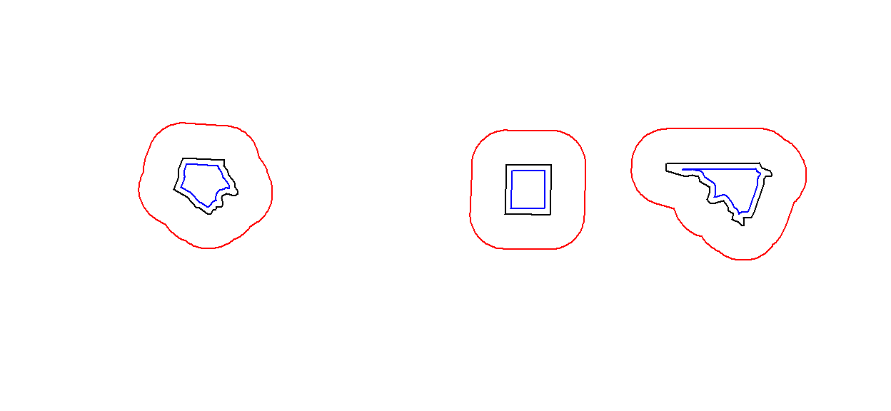
[5,] FALSE FALSE FALSE FALSEThe commands st_buffer, st_boundary, st_convexhull, st_union_cascaded, st_simplify, st_triangulate, st_polygonize, st_centroid, st_segmentize, and st_union return new geometries, e.g.:
sel <- c(1,5,14)
geom = st_geometry(nc.web_mercator[sel,])
buf <- st_buffer(geom, dist = 30000)
plot(buf, border = 'red')
plot(geom, add = TRUE)
plot(st_buffer(geom, -5000), add = TRUE, border = 'blue')
Commands st_intersection, st_union, st_difference, st_sym_difference return new geometries that are a function of pairs of geometries:
The following code shows how computing an intersection between two polygons may yield a GEOMETRYCOLLECTION with a point, line and polygon:
opar <- par(mfrow = c(1, 2))
a <- st_polygon(list(cbind(c(0,0,7.5,7.5,0),c(0,-1,-1,0,0))))
b <- st_polygon(list(cbind(c(0,1,2,3,4,5,6,7,7,0),c(1,0,.5,0,0,0.5,-0.5,-0.5,1,1))))
plot(a, ylim = c(-1,1))
title("intersecting two polygons:")
plot(b, add = TRUE, border = 'red')
(i <- st_intersection(a,b))
plot(a, ylim = c(-1,1))
title("GEOMETRYCOLLECTION")
plot(b, add = TRUE, border = 'red')
plot(i, add = TRUE, col = 'green', lwd = 2)
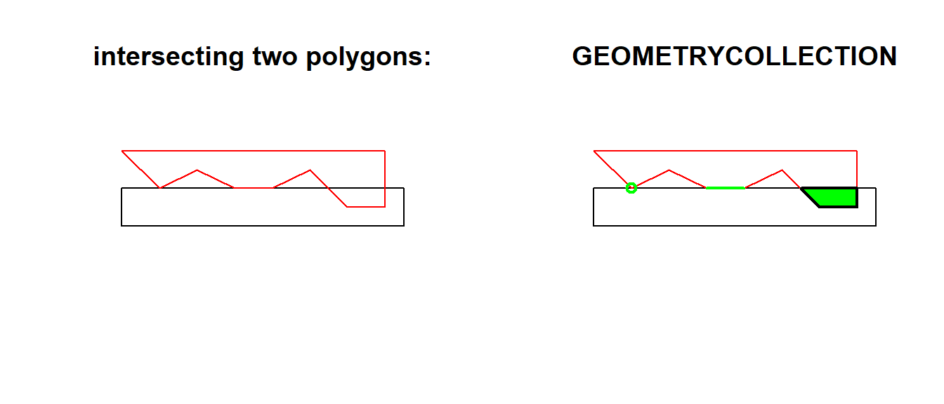
par(opar)
Non-simple and non-valid geometries
Non-simple geometries are for instance self-intersecting lines (left); non-valid geometries are for instance polygons with slivers (middle) or self-intersections (right).
library(sf)
x1 <- st_linestring(cbind(c(0,1,0,1),c(0,1,1,0)))
x2 <- st_polygon(list(cbind(c(0,1,1,1,0,0),c(0,0,1,0.6,1,0))))
x3 <- st_polygon(list(cbind(c(0,1,0,1,0),c(0,1,1,0,0))))
st_is_simple(st_sfc(x1))
[1] FALSEst_is_valid(st_sfc(x2,x3))
[1] FALSE FALSE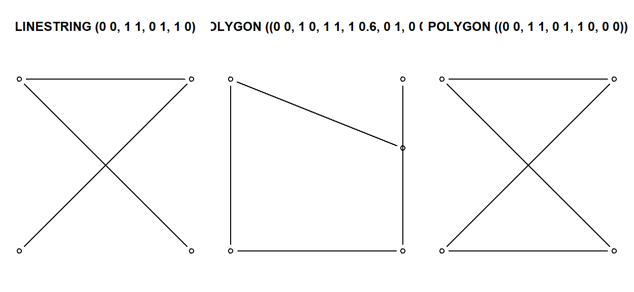
Units
Where possible geometric operations such as st_distance(), st_length() and st_area() report results with a units attribute appropriate for the CRS:
a <- st_area(nc[1,])
attributes(a)
$units
$numerator
[1] "m" "m"

$denominator
character(0)

attr(,"class")
[1] "symbolic_units"

$class
[1] "units"
The units package can be used to convert between units:
units::set_units(a, km^2) # result in square kilometers
1137.389 [km^2]units::set_units(a, ha) # result in hectares
113738.9 [ha]The result can be stripped of their attributes if needs be:
as.numeric(a)
[1] 1137388604How attributes relate to geometries
(This will eventually be the topic of a new vignette; now here to explain the last attribute of sf objects)
The standard documents about simple features are very detailed about the geometric aspects of features, but say nearly nothing about attributes, except that their values should be understood in another reference system (their units of measurement, e.g. as implemented in the package units). But there is more to it. For variables like air temperature, interpolation usually makes sense, for others like human body temperature it doesn’t. The difference is that air temperature is a field, which continues between sensors, where body temperature is an object property that doesn’t extend beyond the body – in spatial statistics bodies would be called a point pattern, their temperature the point marks. For geometries that have a non-zero size (positive length or area), attribute values may refer to the every sub-geometry (every point), or may summarize the geometry. For example, a state’s population density summarizes the whole state, and is not a meaningful estimate of population density for a give point inside the state without the context of the state. On the other hand, land use or geological maps give polygons with constant land use or geology, every point inside the polygon is of that class. Some properties are spatially extensive, meaning that attributes would summed up when two geometries are merged: population is an example. Other properties are spatially intensive, and should be averaged, with population density the example.
Simple feature objects of class sf have an agr attribute that points to the attribute-geometry-relationship, how attributes relate to their geometry. It can be defined at creation time:
nc <- st_read(system.file("shape/nc.shp", package="sf"),
    agr = c(AREA = "aggregate", PERIMETER = "aggregate", CNTY_ = "identity",
        CNTY_ID = "identity", NAME = "identity", FIPS = "identity", FIPSNO = "identity",
        CRESS_ID = "identity", BIR74 = "aggregate", SID74 = "aggregate", NWBIR74 = "aggregate",
        BIR79 = "aggregate", SID79 = "aggregate", NWBIR79 = "aggregate"))
Reading layer `nc' from data source `C:\Users\blancb\Local\R\win-library\4.0\sf\shape\nc.shp' using driver `ESRI Shapefile'
Simple feature collection with 100 features and 14 fields
Attribute-geometry relationship: 0 constant, 8 aggregate, 6 identity
geometry type:  MULTIPOLYGON
dimension:      XY
bbox:           xmin: -84.32385 ymin: 33.88199 xmax: -75.45698 ymax: 36.58965
geographic CRS: NAD27st_agr(nc)
     AREA PERIMETER     CNTY_   CNTY_ID      NAME      FIPS    FIPSNO
aggregate aggregate  identity  identity  identity  identity  identity
 CRESS_ID     BIR74     SID74   NWBIR74     BIR79     SID79   NWBIR79
 identity aggregate aggregate aggregate aggregate aggregate aggregate
Levels: constant aggregate identitydata(meuse, package = "sp")
meuse_sf <- st_as_sf(meuse, coords = c("x", "y"), crs = 28992, agr = "constant")
st_agr(meuse_sf)
 cadmium   copper     lead     zinc     elev     dist       om
constant constant constant constant constant constant constant
   ffreq     soil     lime  landuse   dist.m
constant constant constant constant constant
Levels: constant aggregate identity
When not specified, this field is filled with NA values, but if non-NA, it has one of three possibilities
| value | meaning |
|---|---|
| constant | a variable that has a constant value at every location over a spatial extent; examples: soil type, climate zone, land use |
| aggregate | values are summary values (aggregates) over the geometry, e.g. population density, dominant land use |
| identity | values identify the geometry: they refer to (the whole of) this and only this geometry |
With this information (still to be done) we can for instance
- either return missing values or generate warnings when a aggregate value at a point location inside a polygon is retrieved, or
- list the implicit assumptions made when retrieving attribute values at points inside a polygon when
relation_to_geometryis missing. - decide what to do with attributes when a geometry is split: do nothing in case the attribute is constant, give an error or warning in case it is an aggregate, change the
relation_to_geometryto constant in case it was identity.
Further reading:
I recommend skimming the other articles (#2-#6) on the sf documentation website. They go in depth on contents covered in article #1 copied above.
Leaflet
Acknowledgment: This portion of this module heavily draws upon, including direct copy-paste of markdown content, the the documentation website developed for the leaflet package.
Introduction
Leaflet is one of the most popular open-source JavaScript libraries for interactive maps. It’s used by websites ranging from The New York Times and The Washington Post to GitHub and Flickr, as well as GIS specialists like OpenStreetMap, Mapbox, and CartoDB.
This R package makes it easy to integrate and control Leaflet maps in R.
Features
- Interactive panning/zooming
- Compose maps using arbitrary combinations of:
- Map tiles
- Markers
- Polygons
- Lines
- Popups
- GeoJSON
- Create maps right from the R console or RStudio
- Embed maps in knitr/R Markdown documents and Shiny apps
- Easily render spatial objects from the
sporsfpackages, or data frames with latitude/longitude columns - Use map bounds and mouse events to drive Shiny logic
- Display maps in non spherical mercator projections
- Augment map features using chosen plugins from leaflet plugins repository
Installation
To install this R package, run install.packages("leaflet") command at your R prompt. Once installed, you can use this package at the R console, within R Markdown documents, and within Shiny applications.
Basic Usage
You create a Leaflet map with these basic steps:
- Create a map widget by calling
leaflet(). - Add layers (i.e., features) to the map by using layer functions (e.g.
addTiles,addMarkers,addPolygons) to modify the map widget. - Repeat step 2 as desired.
- Print the map widget to display it.
Here’s a basic example:
library(leaflet)
m <- leaflet() %>%
  addTiles() %>%  # Add default OpenStreetMap map tiles
  addMarkers(lng=174.768, lat=-36.852, popup="The birthplace of R")
m  # Print the map
The Map Widget
The function leaflet() returns a Leaflet map widget, which stores a list of objects that can be modified or updated later. Most functions in this package have an argument map as their first argument, which makes it easy to use the pipe operator %>% in the magrittr package, as you have seen from the example in the Introduction.
Initializing Options
The map widget can be initialized with certain parameters. This is achieved by populating the options argument as shown below.
# Set value for the minZoom and maxZoom settings.
leaflet(options = leafletOptions(minZoom = 0, maxZoom = 18))
The leafletOptions() can be passed any option described in the leaflet reference document. Using the leafletOptions(), you can set a custom CRS and have your map displayed in a non spherical mercator projection as described in projections.
Map Methods
You can manipulate the attributes of the map widget using a series of methods. Please see the help page ?setView for details.
setView()sets the center of the map view and the zoom level;fitBounds()fits the view into the rectangle[lng1, lat1]–[lng2, lat2];clearBounds()clears the bound, so that the view will be automatically determined by the range of latitude/longitude data in the map layers if provided;
The Data Object
Both leaflet() and the map layer functions have an optional data parameter that is designed to receive spatial data in one of several forms:
- From base R:
- lng/lat matrix
- data frame with lng/lat columns
- From the sp package:
SpatialPoints[DataFrame]Line/LinesSpatialLines[DataFrame]Polygon/PolygonsSpatialPolygons[DataFrame]
- From the maps package:
- the data frame from returned from
map()
- the data frame from returned from
The data argument is used to derive spatial data for functions that need it; for example, if data is a SpatialPolygonsDataFrame object, then calling addPolygons on that map widget will know to add the polygons from that SpatialPolygonsDataFrame.
It is straightforward to derive these variables from sp objects since they always represent spatial data in the same way. On the other hand, for a normal matrix or data frame, any numeric column could potentially contain spatial data. So we resort to guessing based on column names:
- the latitude variable is guessed by looking for columns named
latorlatitude(case-insensitive) - the longitude variable is guessed by looking for
lng,long, orlongitude
You can always explicitly identify latitude/longitude columns by providing lng and lat arguments to the layer function.
For example, we do not specify the values for the arguments lat and lng in addCircles() below, but the columns Lat and Long in the data frame df will be automatically used:
# add some circles to a map
df = data.frame(Lat = 1:10, Long = rnorm(10))
leaflet(df) %>% addCircles()
You can also explicitly specify the Lat and Long columns (see below for more info on the ~ syntax):
leaflet(df) %>% addCircles(lng = ~Long, lat = ~Lat)
A map layer may use a different data object to override the data provided in leaflet(). We can rewrite the above example as:
leaflet() %>% addCircles(data = df)
leaflet() %>% addCircles(data = df, lat = ~ Lat, lng = ~ Long)
Below are examples of using sf:
#TODO
The Formula Interface
The arguments of all layer functions can take normal R objects, such as a numeric vector for the lat argument, or a character vector of colors for the color argument. They can also take a one-sided formula, in which case the formula will be evaluated using the data argument as the environment. For example, ~ x means the variable x in the data object, and you can write arbitrary expressions on the right-hand side, e.g., ~ sqrt(x + 1).
m = leaflet() %>% addTiles()
df = data.frame(
  lat = rnorm(100),
  lng = rnorm(100),
  size = runif(100, 5, 20),
  color = sample(colors(), 100)
)
m = leaflet(df) %>% addTiles()
m %>% addCircleMarkers(radius = ~size, color = ~color, fill = FALSE)
m %>% addCircleMarkers(radius = runif(100, 4, 10), color = c('red'))
Markers
Use markers to call out points on the map. Marker locations are expressed in latitude/longitude coordinates, and can either appear as icons or as circles.
Data sources
Point data for markers can come from a variety of sources:
SpatialPointsorSpatialPointsDataFrameobjects (from thesppackage)POINT,sfc_POINT, andsfobjects (from thesfpackage); onlyXandYdimensions will be considered- Two-column numeric matrices (first column is longitude, second is latitude)
- Data frame with latitude and logitude columns. You can explicitly tell the marker function which columns contain the coordinate data (e.g.
addMarkers(lng = ~Longitude, lat = ~Latitude)), or let the function look for columns namedlat/latitudeandlon/lng/long/longitude(case insensitive). - Simply provide numeric vectors as
lngandlatarguments
Note that MULTIPOINT objects from sf are not supported at this time.
Icon Markers
Icon markers are added using the addMarkers or the addAwesomeMarkers functions. Their default appearance is a dropped pin. As with most layer functions, the popup argument can be used to add a message to be displayed on click, and the label option can be used to display a text label either on hover or statically.
data(quakes)
# Show first 20 rows from the `quakes` dataset
leaflet(data = quakes[1:20,]) %>% addTiles() %>%
  addMarkers(~long, ~lat, popup = ~as.character(mag), label = ~as.character(mag))
Customizing Marker Icons
You can provide custom markers in one of several ways, depending on the scenario. For each of these ways, the icon can be provided as either a URL or as a file path.
For the simple case of applying a single icon to a set of markers, use makeIcon().
greenLeafIcon <- makeIcon(
  iconUrl = "http://leafletjs.com/examples/custom-icons/leaf-green.png",
  iconWidth = 38, iconHeight = 95,
  iconAnchorX = 22, iconAnchorY = 94,
  shadowUrl = "http://leafletjs.com/examples/custom-icons/leaf-shadow.png",
  shadowWidth = 50, shadowHeight = 64,
  shadowAnchorX = 4, shadowAnchorY = 62
)
leaflet(data = quakes[1:4,]) %>% addTiles() %>%
  addMarkers(~long, ~lat, icon = greenLeafIcon)
If you have several icons to apply that vary only by a couple of parameters (i.e. they share the same size and anchor points but have different URLs), use the icons() function. icons() performs similarly to data.frame(), in that any arguments that are shorter than the number of markers will be recycled to fit.
quakes1 <- quakes[1:10,]
leafIcons <- icons(
  iconUrl = ifelse(quakes1$mag < 4.6,
    "http://leafletjs.com/examples/custom-icons/leaf-green.png",
    "http://leafletjs.com/examples/custom-icons/leaf-red.png"
  ),
  iconWidth = 38, iconHeight = 95,
  iconAnchorX = 22, iconAnchorY = 94,
  shadowUrl = "http://leafletjs.com/examples/custom-icons/leaf-shadow.png",
  shadowWidth = 50, shadowHeight = 64,
  shadowAnchorX = 4, shadowAnchorY = 62
)
leaflet(data = quakes1) %>% addTiles() %>%
  addMarkers(~long, ~lat, icon = leafIcons)
Finally, if you have a set of icons that vary in multiple parameters, it may be more convenient to use the iconList() function. It lets you create a list of (named or unnamed) makeIcon() icons, and select from that list by position or name.
# Make a list of icons. We'll index into it based on name.
oceanIcons <- iconList(
  ship = makeIcon("ferry-18.png", "ferry-18@2x.png", 18, 18),
  pirate = makeIcon("danger-24.png", "danger-24@2x.png", 24, 24)
)
# Some fake data
df <- sp::SpatialPointsDataFrame(
  cbind(
    (runif(20) - .5) * 10 - 90.620130,  # lng
    (runif(20) - .5) * 3.8 + 25.638077  # lat
  ),
  data.frame(type = factor(
    ifelse(runif(20) > 0.75, "pirate", "ship"),
    c("ship", "pirate")
  ))
)
leaflet(df) %>% addTiles() %>%
  # Select from oceanIcons based on df$type
  addMarkers(icon = ~oceanIcons[type])
Awesome Icons
Leaflet supports even more customizable markers using the awesome markers leaflet plugin.
The addAwesomeMarkers() function is similar to addMarkers() function but additionally allows you to specify custom colors for the markers as well as icons from the Font Awesome, Bootstrap Glyphicons, and Ion icons icon libraries.
Similar to the makeIcon, icons, and iconList functions described above, you have makeAwesomeIcon, awesomeIcons and awesomeIconList functions, which enable you to add awesome icons.
# first 20 quakes
df.20 <- quakes[1:20,]
getColor <- function(quakes) {
  sapply(quakes$mag, function(mag) {
  if(mag <= 4) {
    "green"
  } else if(mag <= 5) {
    "orange"
  } else {
    "red"
  } })
}
icons <- awesomeIcons(
  icon = 'ios-close',
  iconColor = 'black',
  library = 'ion',
  markerColor = getColor(df.20)
)
leaflet(df.20) %>% addTiles() %>%
  addAwesomeMarkers(~long, ~lat, icon=icons, label=~as.character(mag))
The library argument has to be one of ‘ion’, ‘fa’, or ‘glyphicon’. The icon argument needs to be the name of any valid icon supported by the the respective library (w/o the prefix of the library name).
Marker Clusters
When there are a large number of markers on a map, you can cluster them using the Leaflet.markercluster plug-in. To enable this plug-in, you can provide a list of options to the argument clusterOptions, e.g.
leaflet(quakes) %>% addTiles() %>% addMarkers(
  clusterOptions = markerClusterOptions()
)
Using the freezeAtZoom argument of the markerClusterOptions() function you can set the clustering to freeze as a specific zoom level. For example markerClusterOptions(freezeAtZoom = 5) will freeze the cluster at zoom level 5 regardless of the user’s actual zoom level.
Circle Markers
Circle markers are much like regular circles (see Lines and Shapes), except that their radius in onscreen pixels stays constant regardless of zoom level.
You can use their default appearance:
leaflet(df) %>% addTiles() %>% addCircleMarkers()
Or customize their color, radius, stroke, opacity, etc.
# Create a palette that maps factor levels to colors
pal <- colorFactor(c("navy", "red"), domain = c("ship", "pirate"))
leaflet(df) %>% addTiles() %>%
  addCircleMarkers(
    radius = ~ifelse(type == "ship", 6, 10),
    color = ~pal(type),
    stroke = FALSE, fillOpacity = 0.5
  )
Popups
Popups are small boxes containing arbitrary HTML, that point to a specific point on the map.
Use the addPopups() function to add standalone popup to the map.
content <- paste(sep = "<br/>",
  "<b><a href='http://www.samurainoodle.com'>Samurai Noodle</a></b>",
  "606 5th Ave. S",
  "Seattle, WA 98138"
)
leaflet() %>% addTiles() %>%
  addPopups(-122.327298, 47.597131, content,
    options = popupOptions(closeButton = FALSE)
  )
A common use for popups is to have them appear when markers or shapes are clicked. Marker and shape functions in the Leaflet package take a popup argument, where you can pass in HTML to easily attach a simple popup.
library(htmltools)
df <- read.csv(textConnection(
"Name,Lat,Long
Samurai Noodle,47.597131,-122.327298
Kukai Ramen,47.6154,-122.327157
Tsukushinbo,47.59987,-122.326726"
))
leaflet(df) %>% addTiles() %>%
  addMarkers(~Long, ~Lat, popup = ~htmlEscape(Name))
In the preceding example, htmltools::htmlEscape was used to santize any characters in the name that might be interpreted as HTML. While it wasn’t necessary for this example (as the restaurant names contained no HTML markup), doing so is important in any situation where the data may come from a file or database, or from the user.
In addition to markers you can also add popups on shapes like lines, circles and other polygons.
Labels
A label is a textual or HTML content that can attached to markers and shapes to be always displayed or displayed on mouse over. Unlike popups you don’t need to click a marker/polygon for the label to be shown.
library(htmltools)
df <- read.csv(textConnection(
"Name,Lat,Long
Samurai Noodle,47.597131,-122.327298
Kukai Ramen,47.6154,-122.327157
Tsukushinbo,47.59987,-122.326726"))
leaflet(df) %>% addTiles() %>%
  addMarkers(~Long, ~Lat, label = ~htmlEscape(Name))
Customizing Marker Labels
You can customize marker labels using the labelOptions argument of the addMarkers function. The labelOptions argument can be populated using the labelOptions() function. If noHide is false (the default) then the label is displayed only when you hover the mouse over the marker; if noHide is set to true then the label is always displayed.
# Change Text Size and text Only and also a custom CSS
leaflet() %>% addTiles() %>% setView(-118.456554, 34.09, 13) %>%
  addMarkers(
    lng = -118.456554, lat = 34.105,
    label = "Default Label",
    labelOptions = labelOptions(noHide = T)) %>%
  addMarkers(
    lng = -118.456554, lat = 34.095,
    label = "Label w/o surrounding box",
    labelOptions = labelOptions(noHide = T, textOnly = TRUE)) %>%
  addMarkers(
    lng = -118.456554, lat = 34.085,
    label = "label w/ textsize 15px",
    labelOptions = labelOptions(noHide = T, textsize = "15px")) %>%
  addMarkers(
    lng = -118.456554, lat = 34.075,
    label = "Label w/ custom CSS style",
    labelOptions = labelOptions(noHide = T, direction = "bottom",
      style = list(
        "color" = "red",
        "font-family" = "serif",
        "font-style" = "italic",
        "box-shadow" = "3px 3px rgba(0,0,0,0.25)",
        "font-size" = "12px",
        "border-color" = "rgba(0,0,0,0.5)"
      )))
Labels without markers
You can create labels without the accompanying markers using the addLabelOnlyMarkers function.
Lines and Shapes
Leaflet makes it easy to take spatial lines and shapes from R and add them to maps.
Polygons and Polylines
Line and polygon data can come from a variety of sources:
SpatialPolygons,SpatialPolygonsDataFrame,Polygons, andPolygonobjects (from thesppackage)SpatialLines,SpatialLinesDataFrame,Lines, andLineobjects (from thesppackage)MULTIPOLYGON,POLYGON,MULTILINESTRING, andLINESTRINGobjects (from thesfpackage)mapobjects (from themapspackage’smap()function); usemap(fill = TRUE)for polygons,FALSEfor polylines- Two-column numeric matrix; the first column is longitude and the second is latitude. Polygons are separated by rows of
(NA, NA). It is not possible to represent multi-polygons nor polygons with holes using this method; useSpatialPolygonsinstead.
library(rgdal)
# From https://www.census.gov/geo/maps-data/data/cbf/cbf_state.html
states <- readOGR("data/shp/cb_2013_us_state_20m.shp",
  layer = "cb_2013_us_state_20m", GDAL1_integer64_policy = TRUE)
OGR data source with driver: ESRI Shapefile
Source: "C:\Users\blancb\OneDrive - Perkins and Will\Documents\Internal\R Training\nn_r_training\distill_blog\_posts\2021-01-14-geospatial-data\data\shp\cb_2013_us_state_20m.shp", layer: "cb_2013_us_state_20m"
with 52 features
It has 9 fields
Integer64 fields read as doubles:  ALAND AWATER
neStates <- subset(states, states$STUSPS %in% c(
"CT","ME","MA","NH","RI","VT","NY","NJ","PA"
))
leaflet(neStates) %>%
addPolygons(color = "#444444", weight = 1, smoothFactor = 0.5,
opacity = 1.0, fillOpacity = 0.5,
fillColor = ~colorQuantile("YlOrRd", ALAND)(ALAND),
highlightOptions = highlightOptions(color = "white", weight = 2,
bringToFront = TRUE))
Highlighting shapes
The above example uses the highlightOptions parameter to emphasize the currently moused-over polygon. (The bringToFront = TRUE argument is necessary to prevent the thicker, white border of the active polygon from being hidden behind the borders of other polygons that happen to be higher in the z-order.) You can use highlightOptions with all of the shape layers described on this page.
Circles
Circles are added using addCircles(). Circles are similar to circle markers; the only difference is that circles have their radii specified in meters, while circle markers are specified in pixels. As a result, circles are scaled with the map as the user zooms in and out, while circle markers remain a constant size on the screen regardless of zoom level.
When plotting circles, only the circle centers (and radii) are required, so the set of valid data sources is different than for polygons and the same as for markers. See the introduction to Markers for specifics.
cities <- read.csv(textConnection("
City,Lat,Long,Pop
Boston,42.3601,-71.0589,645966
Hartford,41.7627,-72.6743,125017
New York City,40.7127,-74.0059,8406000
Philadelphia,39.9500,-75.1667,1553000
Pittsburgh,40.4397,-79.9764,305841
Providence,41.8236,-71.4222,177994
"))
leaflet(cities) %>% addTiles() %>%
  addCircles(lng = ~Long, lat = ~Lat, weight = 1,
    radius = ~sqrt(Pop) * 30, popup = ~City
  )
Rectangles
Rectangles are added using the addRectangles() function. It takes lng1, lng2, lat1, and lat2 vector arguments that define the corners of the rectangles. These arguments are always required; the rectangle geometry cannot be inferred from the data object.
leaflet() %>% addTiles() %>%
  addRectangles(
    lng1=-118.456554, lat1=34.078039,
    lng2=-118.436383, lat2=34.062717,
    fillColor = "transparent"
  )
Show/Hide Layers
The Leaflet package includes functions to show and hide map layers. You can allow users to decide what layers to show and hide, or programmatically control the visibility of layers using server-side code in Shiny.
In both cases, the fundamental unit of showing/hiding is the group.
Understanding Groups
A group is a label given to a set of layers. You assign layers to groups by using the group parameter when adding the layers to the map.
leaflet() %>%
  addTiles() %>%
  addMarkers(data = coffee_shops, group = "Food & Drink") %>%
  addMarkers(data = restaurants, group = "Food & Drink") %>%
  addMarkers(data = restrooms, group = "Restrooms")
Many layers can belong to same group. But each layer can only belong to zero or one groups (you can’t assign a layer to two groups).
Groups vs. Layer IDs
Groups and Layer IDs may appear similar, in that both are used to assign a name to a layer. However, they differ in that layer IDs are used to provide a unique identifier to individual markers and shapes, etc., while groups are used to give shared labels to many items.
You generally provide one group value for the entire addMarkers call, and you can reuse that same group value in future addXXX calls to add to that group’s membership (as in the example above).
layerId arguments are always vectorized: when calling e.g. addMarkers you need to provide one layer ID per marker, and they must all be unique. If you add a circle with a layer ID of "foo" and later add a different shape with the same layer ID, the original circle will be removed.
Interactive Layer Display
You can use Leaflet’s layers control feature to allow users to toggle the visibility of groups.
outline <- quakes[chull(quakes$long, quakes$lat),]
map <- leaflet(quakes) %>%
  # Base groups
  addTiles(group = "OSM (default)") %>%
  addProviderTiles(providers$Stamen.Toner, group = "Toner") %>%
  addProviderTiles(providers$Stamen.TonerLite, group = "Toner Lite") %>%
  # Overlay groups
  addCircles(~long, ~lat, ~10^mag/5, stroke = F, group = "Quakes") %>%
  addPolygons(data = outline, lng = ~long, lat = ~lat,
    fill = F, weight = 2, color = "#FFFFCC", group = "Outline") %>%
  # Layers control
  addLayersControl(
    baseGroups = c("OSM (default)", "Toner", "Toner Lite"),
    overlayGroups = c("Quakes", "Outline"),
    options = layersControlOptions(collapsed = FALSE)
  )
map
The addLayersControl function distinguishes between base groups, which can only be viewed one group at a time, and overlay groups, which can be individually checked or unchecked.
Although base groups are generally tile layers, and overlay groups are usually markers and shapes, there is no restriction on what types of layers can be placed in each category.
Only one layers control can be present on a map at a time. If you call addLayersControl multiple times, the last call will win.
Programmatic Layer Display
You can use the showGroup and hideGroup functions to show and hide groups from code. This mostly makes sense in a Shiny context with leafletProxy, where perhaps you might toggle group visibility based on input controls in a sidebar.
You can also use showGroup/hideGroup in conjuction with addLayersControl to set which groups are checked by default.
map %>% hideGroup("Outline")
Example
Using the skills learned above, we are going to load in Excel data for Nelson\Nygaard’s projects and offices, and translate those into geospatial data, and perform some simple geocomputations using buffers and intersections. Then we will map the data using leaflet, and plot a simple summary using ggplot.
Notes on below code:
Coordinate System Reference Codes: You will want to get comfortable using the EPSG codes for different coordinate systems, as that is the easiest way to reference them in R/sf. The website I use to find the appropriate EPSG code for a given area is spatialreference.org. You will typically have to use this when using different state plane coordinate systems from different parts of the country. It is always handy to remember that WGS84 (the master geographic coordinate system for the globe in latitude & longitude) can be referenced by EPSG code
4326, as is used below.Seamless work with spatial and non-spatial attributes: One of the greatest features of the
sfpackage is how seamlessly it integrates into the tidyverse. Just as we can do spatial operations below, we can also use tidyverse methods likeggplot()to create summaries that rely on spatial computations (in this case, an intersection).
#Load in packages
library(tidyverse)
library(sf)
library(readxl)
library(janitor)
library(leaflet)

#Read in Excel files
project_cities = read_excel('data/Projects_MASTER.xlsx',sheet='GISJOIN_202004')
nn_offices = read_excel('data/Projects_MASTER.xlsx',sheet='nn_offices')

#Add geometry to project cities using st_as_sf() function
project_cities_sf = project_cities %>%
  clean_names() %>%
  #Filter out international projects
  filter(is.na(international)) %>%
  #Select columns of interest
  select(city,state,x,y,all:other) %>%
  #Can turn data frame into sf data frame by referencing coordinates (for points)
  st_as_sf(coords = c('x','y'),crs = 4326)

#Same as above
nn_offices_sf = nn_offices %>%
  clean_names() %>%
  st_as_sf(coords = c('x','y'),crs=4326)

#Making custom NN icon based on JPEG image stored on website.
nn_icon = makeIcon(iconUrl = 'https://perkinsandwill.github.io/nn_r_training/topics_setup/03_geospatial/graphics/NNlogo_RGB_300dpi_JPEG.jpg',
                   #Making icon 10% of original size
                   iconWidth = 331*0.1,
                   iconHeight = 450*0.1,
                   #Anchor point at center of icon (halfway in X and Y)
                   iconAnchorX = 331*0.1*0.5,
                   iconAnchorY = 450*0.1*0.5)

#Basic map showing offices as icons (icon assembled above)
leaflet() %>%
  addProviderTiles('CartoDB.Positron') %>%
  addMarkers(data =nn_offices_sf,icon = nn_icon,
             #Using formula notation, as discussed above, can reference attributes
             label=~city)
nn_office_buffers = nn_offices_sf %>%
  #Going to use Oregon North (2269) even though this will be slightly inaccurate with a nationwide buffer calculation
  st_transform(2269) %>%
  #Create fifty mile buffer
  st_buffer(5280*50) %>%
  #Transform back to WGS84
  st_transform(4326)

#Basic map showing buffer polygons
leaflet() %>%
  addProviderTiles('CartoDB.Positron') %>%
  addPolygons(data = nn_office_buffers,
              label=~city)
#Using Intersection to group project cities within 50 miles of an office.
sub_project_cities_sf = project_cities_sf %>%
  #Intersection only operates with planar coordinates, need to transform to state plane temporarily
  st_transform(2269) %>%
  #Intersecting with office buffers
  st_intersection(nn_office_buffers %>%
                    select(nn_office_id,city,geometry) %>%
                    rename(office_city = city) %>%
                    st_transform(2269)) %>%
  #Transform back for mapping
  st_transform(4326)

#Mapping offices and project cities using groups and layer control.
#Sizing circle markers for project cities by number of projects.
leaflet() %>%
  addProviderTiles('CartoDB.DarkMatter') %>%
  addMarkers(data =nn_offices_sf,icon = nn_icon,
             label=~city,group=~city) %>%
  addCircleMarkers(data=sub_project_cities_sf,
                   radius=~all*1.5, label=~paste0(city,": ",all,' projects'),
                   group=~office_city,
                   fillOpacity = 0.7,color='white',opacity =0.9,
                   fillColor = '#00659A',weight=3) %>%
  addLayersControl(baseGroups = unique(sub_project_cities_sf$office_city))
#Create a summary for plotting
summ_project_cities_by_office = sub_project_cities_sf %>%
#Use the as_tibble() function to get rid of sf features -- otherwise geometries will not come off in select function.
as_tibble() %>%
select(office_city,transit:other) %>%
#pivot by project type
pivot_longer(transit:other,names_to='sector',values_to='num_projects') %>%
#filter out project types where num_projects is 0
filter(num_projects>0) %>%
group_by(office_city) %>%
#computed proportion of projects for second of below plots
mutate(prop_projects = num_projects/sum(num_projects))
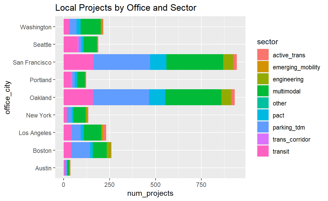
#Plot projects by office and sector
ggplot(summ_project_cities_by_office,
aes(x=office_city,y=num_projects,fill=sector))+
geom_col()+
coord_flip()+
ggtitle('Local Projects by Office and Sector')
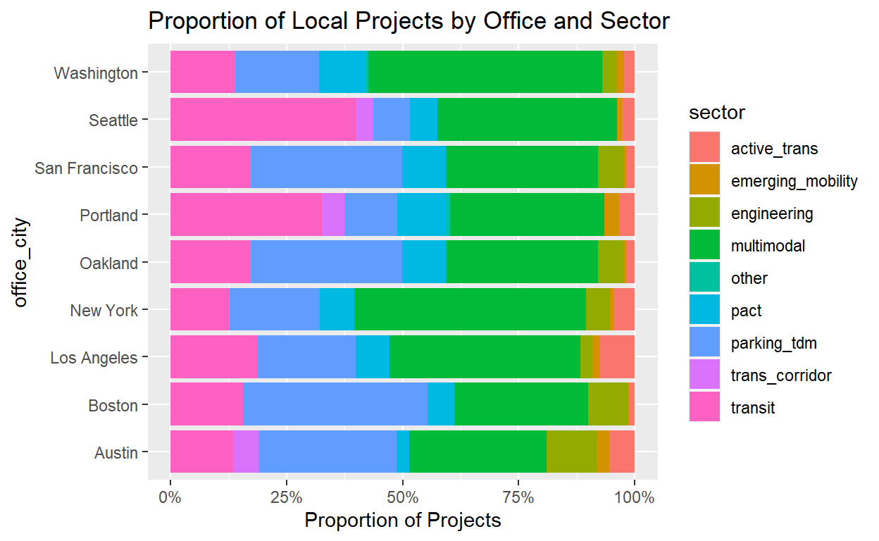
#Use proportion to create a 100% bar plot
ggplot(summ_project_cities_by_office,
       aes(x=office_city,y=prop_projects,fill=sector))+
  geom_col()+
  coord_flip()+
  #Use percent labels function from scales package
  scale_y_continuous(labels=scales::percent,name='Proportion of Projects')+
  ggtitle('Proportion of Local Projects by Office and Sector')
Reference Materials
Further Reading
- Geocomputation with R (web version)
- Applied Spatial Data Analysis with R (PDF version)
- An Introduction to R for Spatial Analysis and Mapping (available where books are sold)
Cheat Sheets
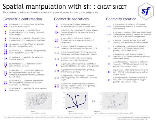
Simple Features (sf) Cheat Sheet
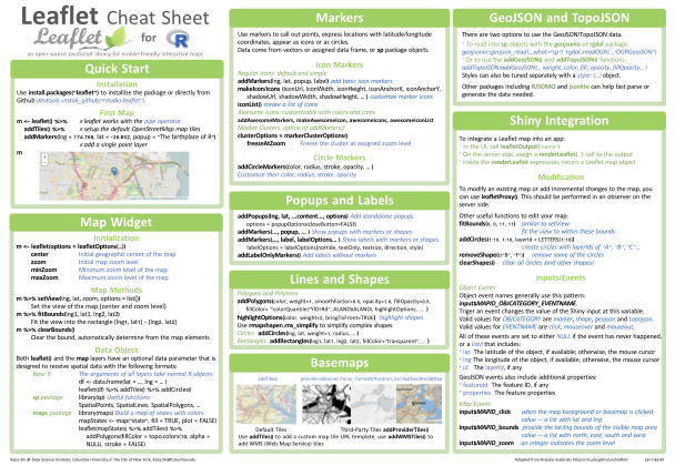
Leaflet for R Cheat Sheet
Related DataCamp Courses
- Spatial data with R (4 courses, 16 hours, includes leaflet course noted below)
- Interactive Maps with leaflet (1 course, 4 hours)
This content was presented to Nelson\Nygaard Staff at a Lunch and Learn webinar on Friday, September 4th, 2020, and is available as a recording here and embedded at the top of this page