Methodology
Setup
To use this on your own network, you will want to make a copy of the scripts/osm-segmentation-script.R file and edit it per the user input adjustments below. The headings within the script follow the step number headings below.
The major data input that you must come to this process with is a GTFS feed. You can generally download the latest GTFS feed from a transit agency’s website, but you can also download historical GTFS feeds from transitfeeds.com. Other than that, the only other things you need are some small metadata inputs, listed below:
app_time_period: You’ll want to name the time period represented by this GTFS feed, especially if you want to use multiple GTFS feeds for the same agency. This can be any character string, but typically will look like"Fall 2022".folder_name: You will want a name for the folder generated for the results – usually this can be the agency name or some abbreviation for it.coord_local: You will want to select the local (planar) coordinate system EPSG code for the agency you are analyzing – you can use this helper Shiny application to select one.feed_path: You will want to download the GTFS feed selected above into the repository in which you are carrying out the segmentation process, and then you need to identify its path for the script to operate.
These inputs can be edited in the section of the USER INPUTS section of the script near the top.
Segmentation Process
The following narrative describes the process carried out for a particular GTFS feed, as laid out in this script. The step numbers below match the step numbers listed in the script so you can consider the code (which has additional comments for clarity) alongside this narrative description.
Depending on the size of the network and the computing resources available, the overall process can take up to 1-2 days to complete, so please plan ahead for your projects. For a small network (e.g., the Lane Transit District in Eugene used in the latest sample version of the script), it can take just a few hours. The vast majority of this time does not require active attention, the script can be running in the background, but you may need to troubleshoot at various junctures to be called out below.
Step 1: Match All Route Shapes to OSM Network Using Valhalla
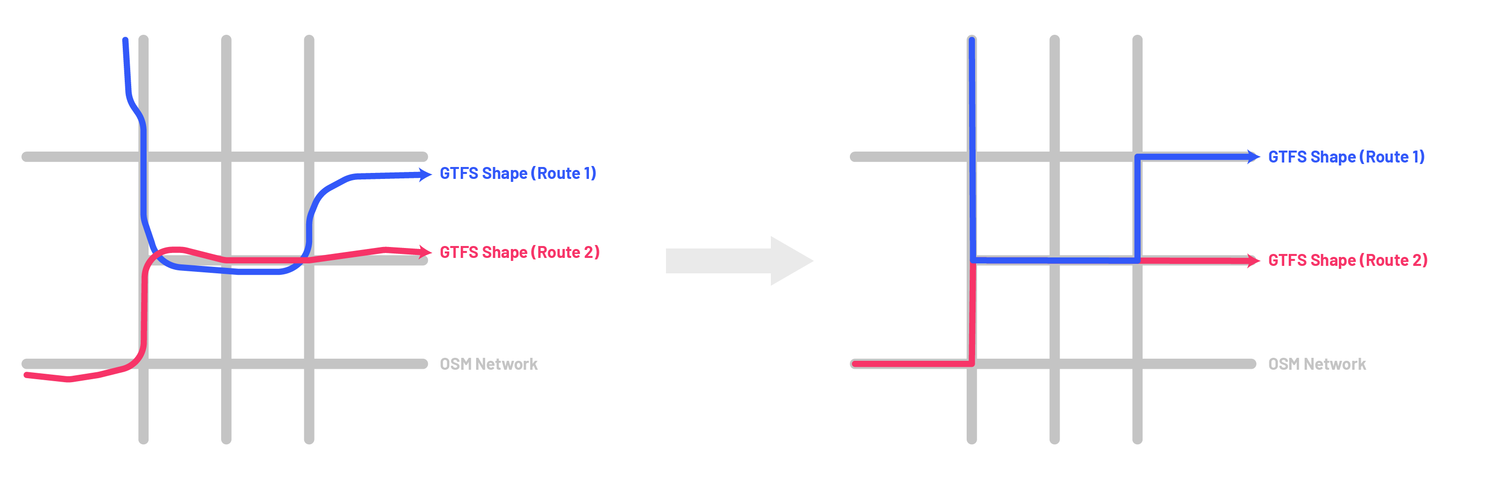
GTFS feeds contain, in the shapes table, a definition (in geographic coordinates) of the geometry for each pattern a route in the feed serves. Using Valhalla (an open source routing machine), we will match each shape in the shapes table to the OSM network. You (most likely) do not need to specify the OSM network to be matched at this point — Nelson\Nygaard’s implementation of Valhalla can match to any OSM network in North America. This process will result in a) a ‘trace’ defining the matched route (i.e. a sequence of geographic coordinates snapped onto the OSM network in the matched route), and b) a sequence of OSM ways that were used to for the matched route. Both will be used in future steps.
Occasionally, your internet connection with the OSM API can be interrupted and the loop can stop unexpectedly – this was observed sporadically during testing. You can simply modify the beginning index of the loop temporarily to start from where the loop left off and continue matching the rest of the routes. We will attempt to resolve this in future versions of this script.
Step 2: Fetch OSM Network Information for Geometry Development
Now that we have the full list of OSM network ways (also referred to as links or edges), we can pull down from OpenStreetMap the ‘universe’ of ways and nodes to consider in developing our segment geometry. As part of this work, I developed a function to pull down, for a given set of OSM ways, the associated network information needed for future steps – a) connected nodes, b) node-to-node relations, and c) way-to-way relations. For a reasonably sized urban area this function will take several hours to run, so please plan ahead when running this process.
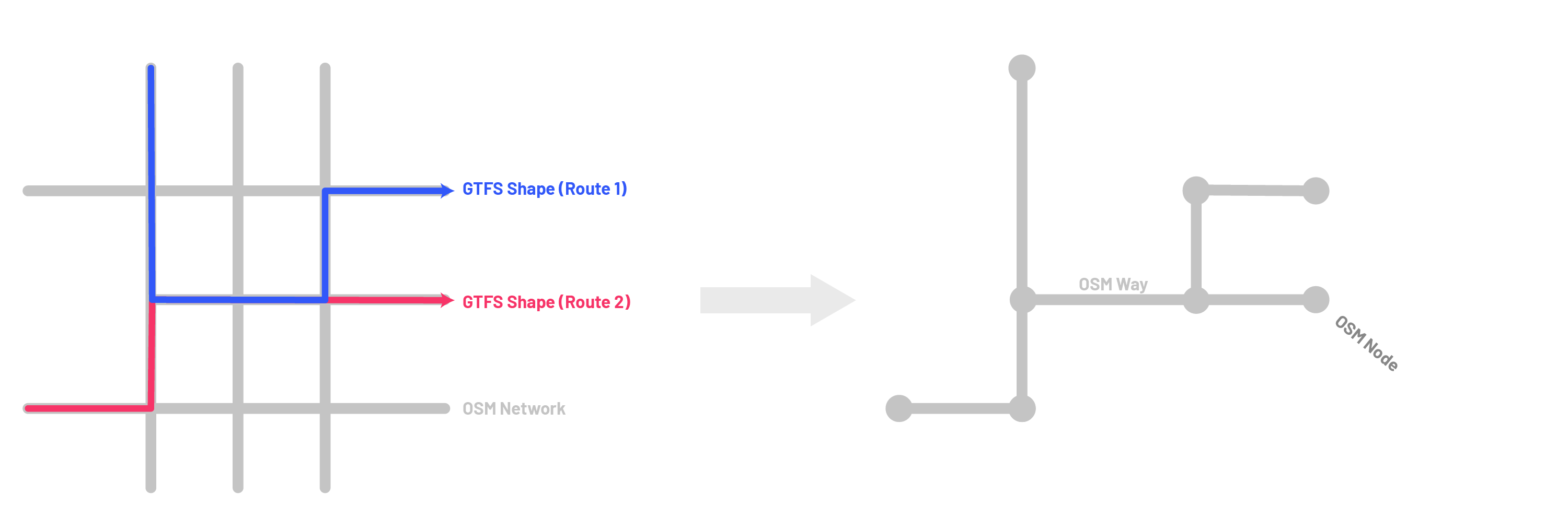
Step 3: Match Valhalla Traces and Way Sequences to Nodes
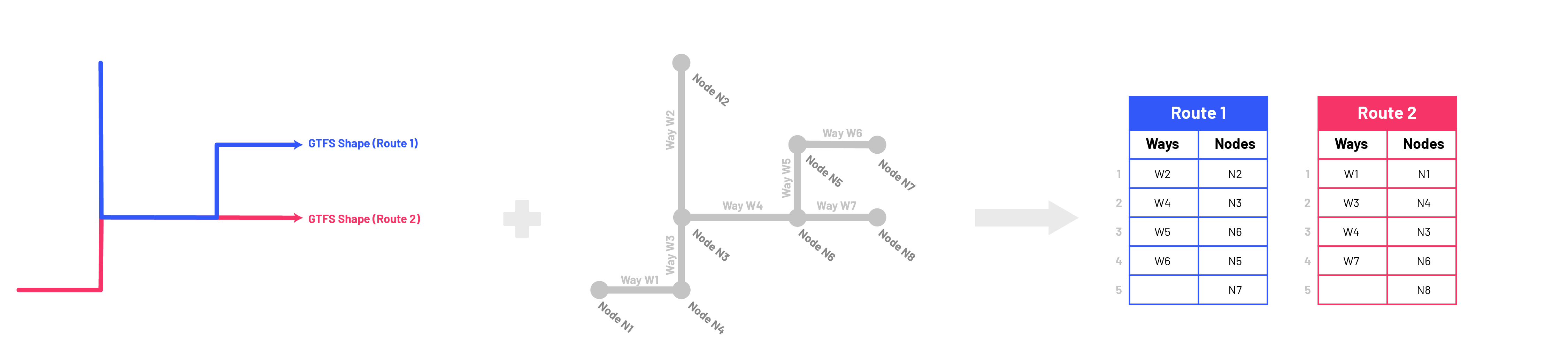
We only received the sequence of OSM ways from Valhalla, so now, using the relations queried in step 2 and Valhalla coordinate trace from step 1, we must identify the OSM nodes used for each route shape (and their sequence). This part of the script uses a loop to carry out this node identification process for each route shape, resulting in a tibble with every node used (in sequence) for each route shape and their relationship to the OSM ways sequence as well.
Step 4: Identify Breakpoints
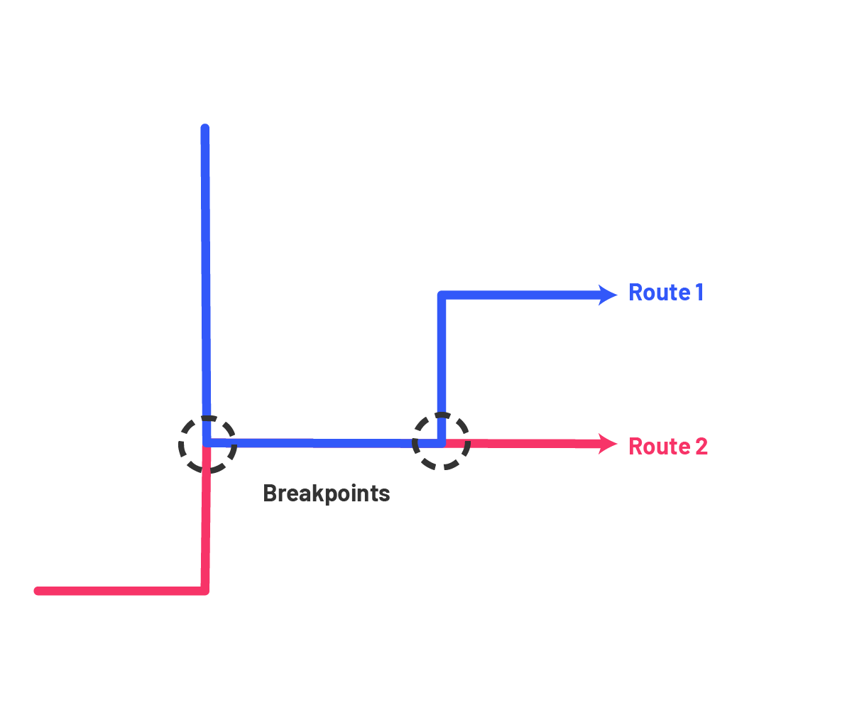
As used in the Austin implementation of this methodology, custom breakpoints can also be developed and utilized as the endpoints between segments, but for the purposes of automating a good first attempt – though it is noted in future steps for this project as an avenue for further development — we will automate the identification of breakpoints based solely on the convergence and divergence of different routes. In the next step we will also break segments based on a typical maximum length but these will not be anchored to specific breakpoints, which are distinct conceptual entities in this methodology.
Step 5: Knit Ways into Segments between Identified Breakpoints
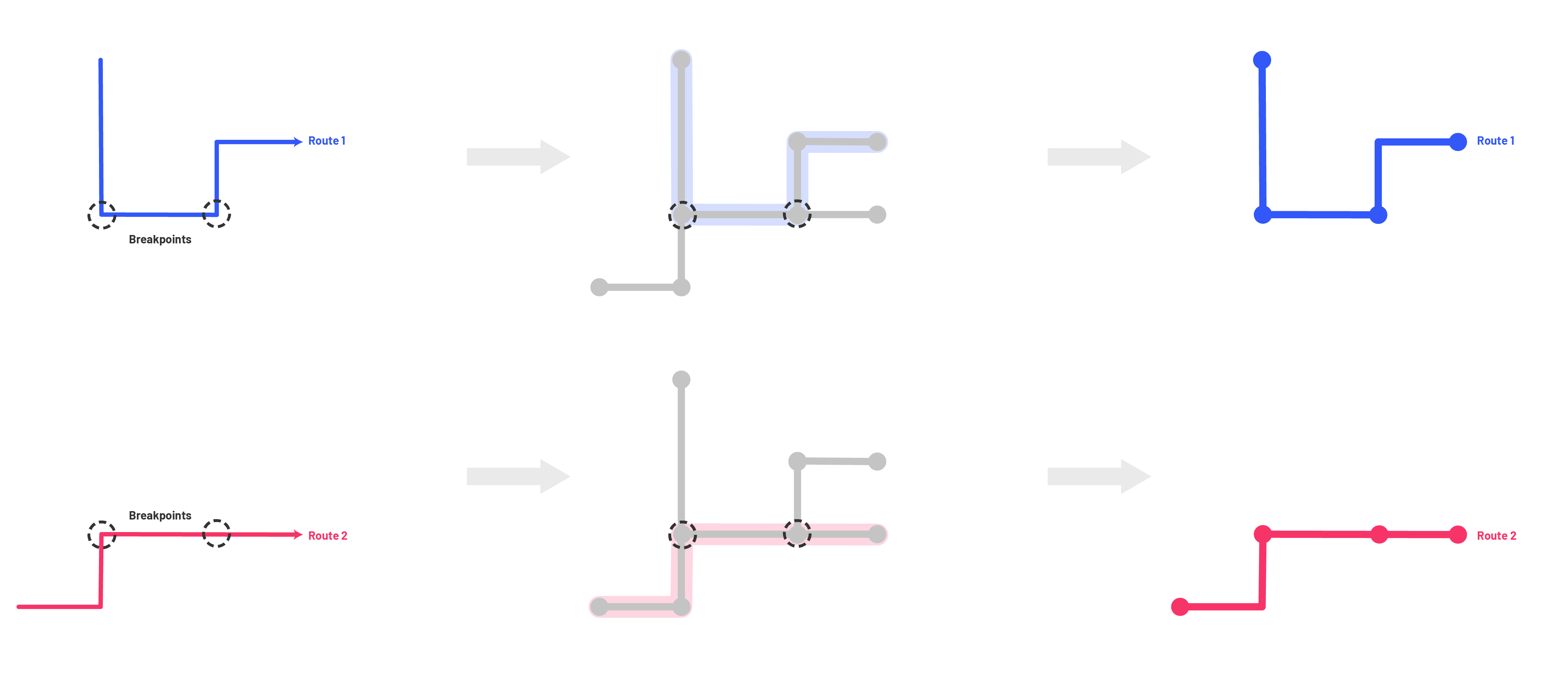
After the identification of breakpoints is complete, we then move on to the most complex part of the process – the cohesion of OSM ways into segments between breakpoints. This is the part of the script where all the preparation work done in previous steps is used to develop the segment geometries. A series of functions is used throughout, and these are independently commented for more thorough explanation.
As mentioned above, we have also implemented in this step an additional way that segments are broken – an ideal maximum length (we have used 1 mile but this can be adjusted easily in the script). This was added because less dense areas of a transit network can sometimes have multiple miles between breakpoints and it is typically desired to have a greater resolution of data than this.
Step 6: Post-Processing and Cleaning for Final Segments and Assignments
Step 5 creates all of the segment geometries independently. In order to minimize the number of distinct segments in the systemwide network, we will use geometric comparison methods to identify identical segment geometries to be merged into a single segment identifier, and segments similar enough to choose a single segment geometry (and identifier) to represent all of them. After this cleaning of redundancies, the segmentation process is finished!
Results
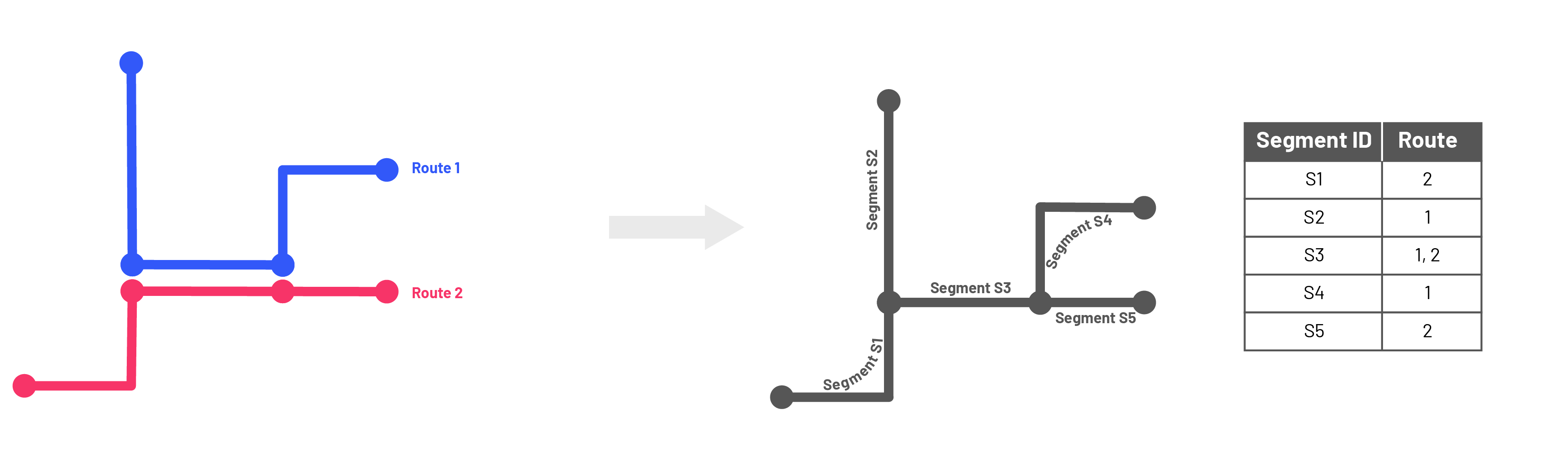
There are two primary resulting datasets from the segmentation process:
- Segment geometries. These are the geometries (
sfLINESTRINGs) corresponding to the resultant segment set. An arbitrary sequence is used for thesegment_id. A key note is that these geometries are intentionally drawn by direction – segments are not bi-directional. This allows for distinguishing data by direction both inside and outside of mapping contexts. - Segment assignments by route shape. Sequenced assignments of segments for each route shape – this table maps the relationships between routes (and their directions and patterns) and segments that is used for aggregating data by segment across routes.
You can view the resulting segment geometries and route assignments from several sample networks in the Shiny demonstration app.
For now, the easiest way to QA/QC the results is to use the demo Shiny app included in the repository (see helper-shiny-apps/osm-segment-review-app for app code), editing the code to use your selected GTFS feed. The segment results can be loaded for this app using th scripts/segment-review-app-etl.R script.