Setup
library(tidyverse)
library(scales)
library(nntools)
library(janitor)
library(gapminder)
library(rnaturalearth)
library(tigris)
library(sf)
library(systemaGlobalis)

sg_country_list <- countries %>%
  mutate(iso_n3 = str_pad(iso3166_1_numeric,side="left",pad="0",width=3))

# concepts_of_interest <- concepts %>%
#   filter(concept %in% c("total_population_with_projections","total_gdp_ppp_inflation_adjusted",
#                         "surface_area_sq_km"))
#
# gm_sub <- datapoints %>%
#   select(geo,time,any_of(concepts_of_interest$concept)) %>%
#   rename(geo_code = geo,year=time) %>%
#   left_join(sg_country_list %>%
#               select(country,iso3166_1_numeric) %>%
#               rename(geo_code = country)) %>%
#   mutate(iso_n3 = str_pad(iso3166_1_numeric,side="left",pad="0",width=3))

world_countries = ne_countries(returnclass = "sf", scale = "medium")

world_region_ref <- world_countries %>%
  st_drop_geometry() %>%
  select(iso_a3, iso_n3, name, region_wb)

pop_total_raw = read_csv("gapminder_data/population_total.csv")
gdp_per_capita_raw = read_csv("gapminder_data/income_per_person_gdppercapita_ppp_inflation_adjusted.csv",
                              col_types = "c")
land_area_raw = read_csv("gapminder_data/ag_lnd_totl_k2.csv")

clean_pop <- pop_total_raw %>%
  pivot_longer(cols = -any_of("country"),names_to = "year",values_to = "pop_est_chr") %>%
  mutate(pop_est = case_when(
    str_detect(pop_est_chr,"k") ~ as.numeric(str_extract(pop_est_chr,"[[:digit:]]+\\.*[[:digit:]]*"))*1e3,
    str_detect(pop_est_chr,"M") ~ as.numeric(str_extract(pop_est_chr,"[[:digit:]]+\\.*[[:digit:]]*"))*1e6,
    str_detect(pop_est_chr,"B") ~ as.numeric(str_extract(pop_est_chr,"[[:digit:]]+\\.*[[:digit:]]*"))*1e9
  )) %>%
  select(-pop_est_chr)

clean_land_area <- land_area_raw %>%
  pivot_longer(cols = -any_of("country"),names_to = "year",values_to = "land_est_chr") %>%
  mutate(land_est_sq_km = case_when(
    str_detect(land_est_chr,"k") ~ as.numeric(str_extract(land_est_chr,"[[:digit:]]+\\.*[[:digit:]]*"))*1e3,
    str_detect(land_est_chr,"M") ~ as.numeric(str_extract(land_est_chr,"[[:digit:]]+\\.*[[:digit:]]*"))*1e6,
    str_detect(land_est_chr,"B") ~ as.numeric(str_extract(land_est_chr,"[[:digit:]]+\\.*[[:digit:]]*"))*1e9,
    TRUE ~ as.numeric(str_extract(land_est_chr,"[[:digit:]]+\\.*[[:digit:]]*"))
  ))  %>%
  select(-land_est_chr)

clean_gdp_per_capita <- gdp_per_capita_raw %>%
  mutate_all(as.character) %>%
  pivot_longer(cols = -any_of("country"),names_to = "year",values_to = "gdp_per_capita_chr")  %>%
  mutate(gdp_per_capita_est = case_when(
    str_detect(gdp_per_capita_chr,"k") ~ as.numeric(str_extract(gdp_per_capita_chr,"[[:digit:]]+\\.*[[:digit:]]*"))*1e3,
    str_detect(gdp_per_capita_chr,"M") ~ as.numeric(str_extract(gdp_per_capita_chr,"[[:digit:]]+\\.*[[:digit:]]*"))*1e6,
    str_detect(gdp_per_capita_chr,"B") ~ as.numeric(str_extract(gdp_per_capita_chr,"[[:digit:]]+\\.*[[:digit:]]*"))*1e9,
    TRUE ~ as.numeric(str_extract(gdp_per_capita_chr,"[[:digit:]]+\\.*[[:digit:]]*"))
  ))  %>%
  select(-gdp_per_capita_chr)

clean_ts_data = clean_pop %>%
  left_join(clean_gdp_per_capita) %>%
  left_join(clean_land_area) %>%
  group_by(country) %>%
  fill(land_est_sq_km, .direction = "downup") %>%
  filter(year <=2021) %>%
  mutate(pop_density = pop_est/land_est_sq_km,
         total_gdp = gdp_per_capita_est*pop_est) %>%
  ungroup() %>%
  mutate(year = as.numeric(year)) %>%
  left_join(sg_country_list %>% select(name,iso_n3) %>%
              rename(country = name)) %>%
  left_join(world_region_ref %>% distinct(iso_n3,region_wb) %>%
              filter(!is.na(iso_n3)))

# clean_ts_data = gm_sub %>%
#   rename(pop_est = total_population_with_projections,
#          land_est_sq_km = surface_area_sq_km,
#          gdp_per_capita_est = total_gdp_ppp_inflation_adjusted) %>%
#   mutate(pop_density = pop_est/land_est_sq_km,
#          total_gdp = gdp_per_capita_est*pop_est) %>%
#   left_join(world_region_ref)
Time Series Plots
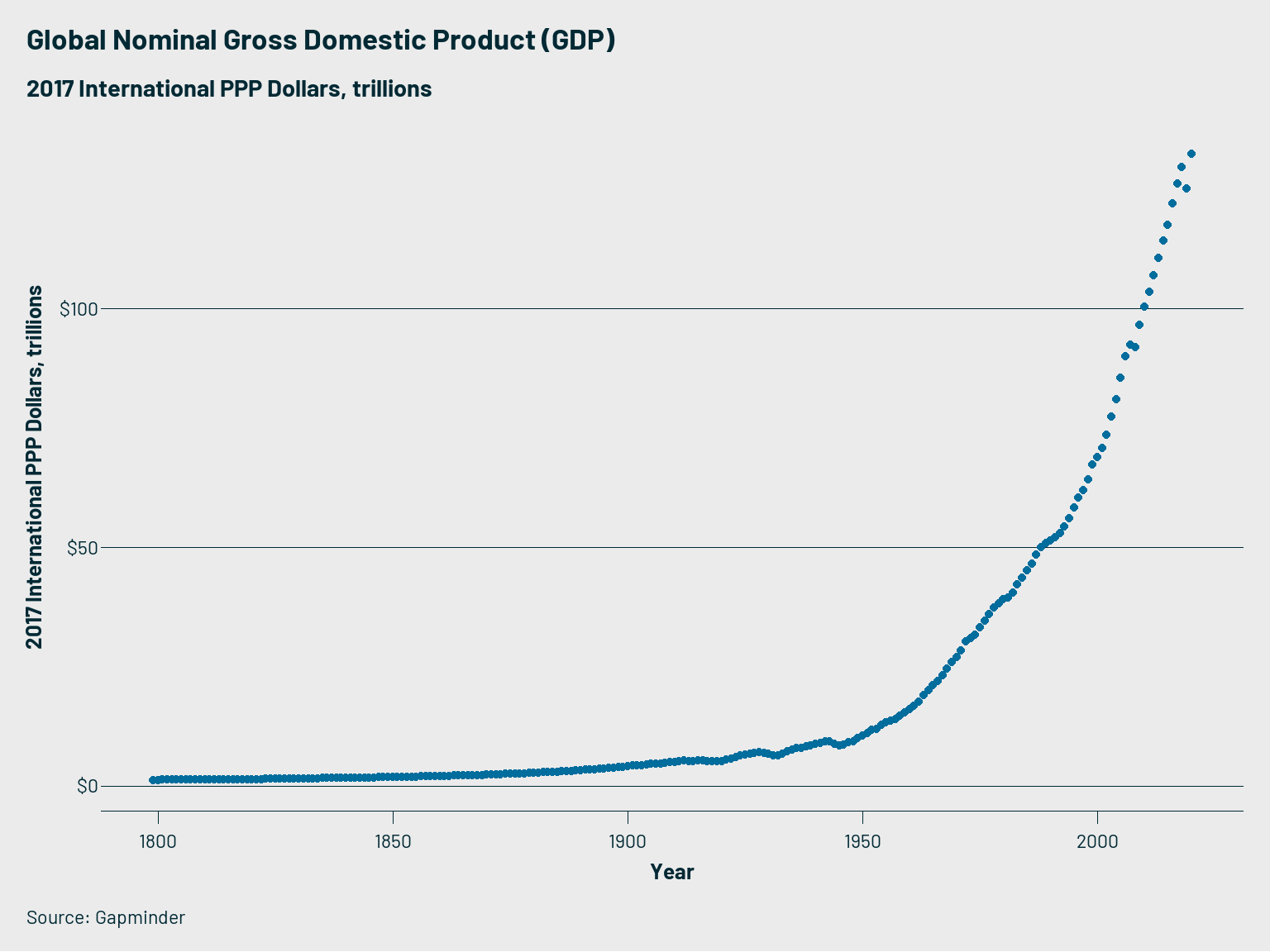
global_gdp <- clean_ts_data %>%
  filter(year <=2020) %>%
  group_by(year) %>%
  summarise(total_gdp = sum(total_gdp,na.rm = TRUE))

ggplot(global_gdp,aes(x=year,y=total_gdp/1e12))+
  geom_point(color = nn_colors("NN Blue"))+
  nn_basic_theme(base_size=22)+
  scale_y_continuous(labels = dollar, name = "2017 International PPP Dollars, trillions")+
  labs(title = "Global Nominal Gross Domestic Product (GDP)",
       subtitle = "2017 International PPP Dollars, trillions",
       caption = "Source: Gapminder",
       x="Year")
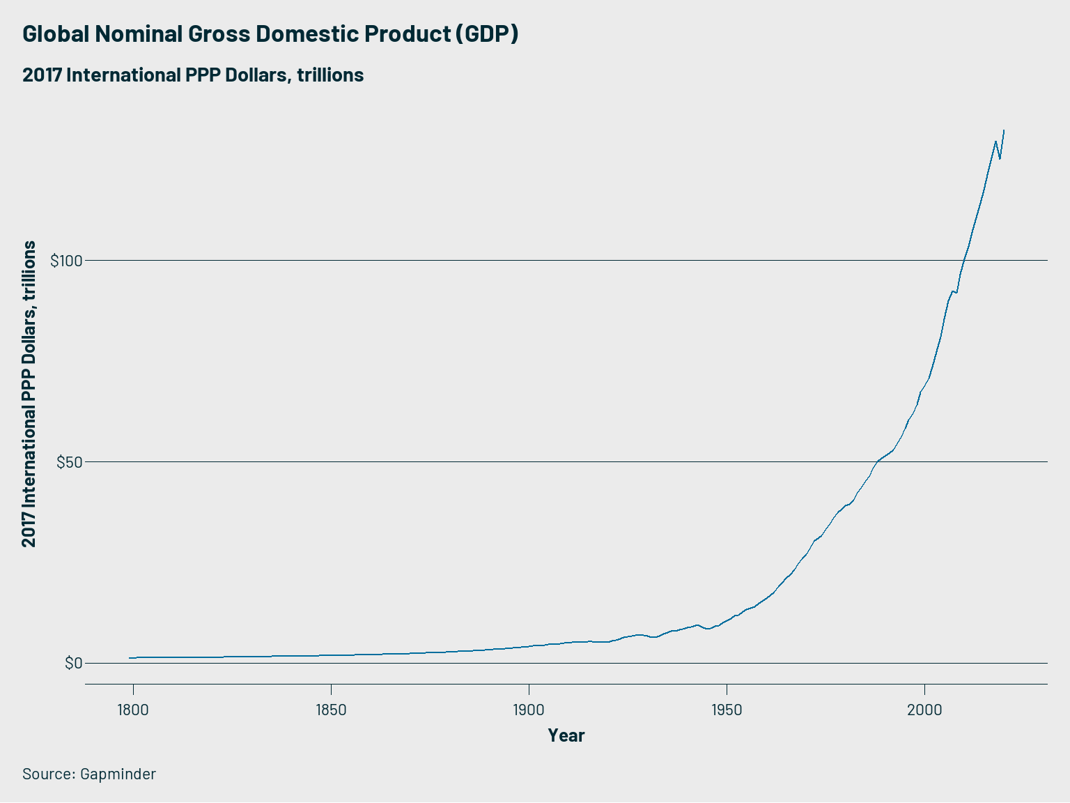
ggplot(global_gdp,aes(x=year,y=total_gdp/1e12))+
  geom_line(color = nn_colors("NN Blue"))+
  nn_basic_theme(base_size=22)+
  scale_y_continuous(labels = dollar, name = "2017 International PPP Dollars, trillions")+
  labs(title = "Global Nominal Gross Domestic Product (GDP)",
       subtitle = "2017 International PPP Dollars, trillions",
       caption = "Source: Gapminder",
       x="Year")
Distribution Plots
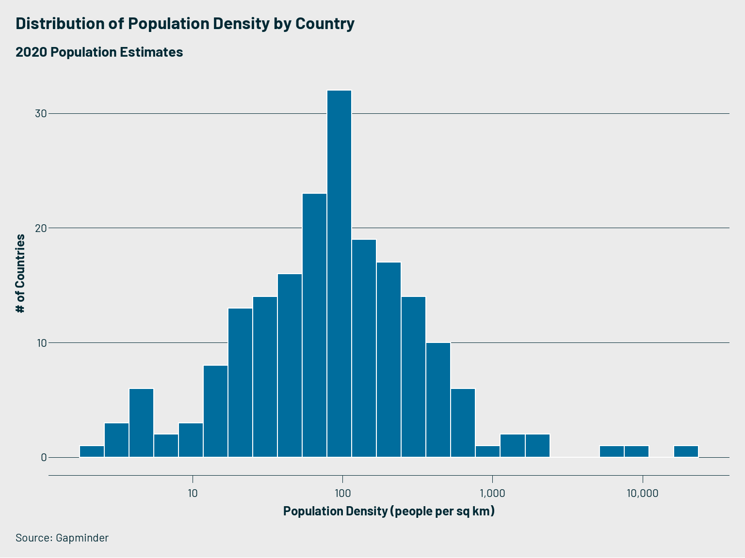
current_pop_densities <- clean_ts_data %>%
  filter(year == 2020)

ggplot(current_pop_densities,aes(x=pop_density))+
  geom_histogram(fill = nn_colors("NN Blue"), bins = 25,
                 color = nn_colors("NN White")) +
  scale_x_log10(labels = comma) +
  nn_basic_theme(base_size=22) +
  labs(title = "Distribution of Population Density by Country",
       subtitle = "2020 Population Estimates",
       caption = "Source: Gapminder",
       y="# of Countries",
       x="Population Density (people per sq km)")
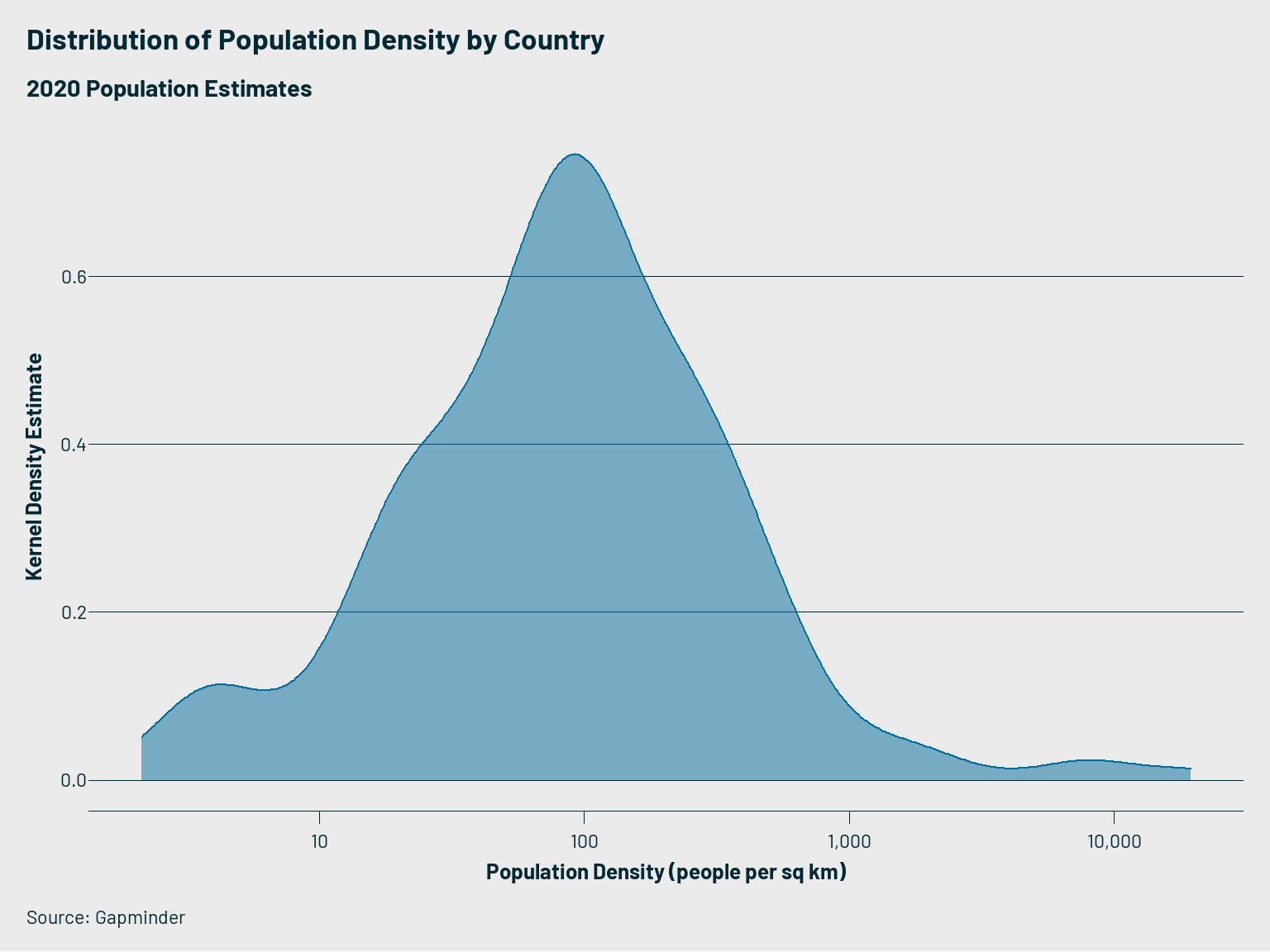
ggplot(current_pop_densities,aes(x=pop_density))+
  geom_density(fill = nn_colors("NN Blue"), alpha=0.5,
               color = nn_colors("NN Blue"))+
  scale_x_log10(labels=comma)+
  nn_basic_theme(base_size=22) +
  labs(title = "Distribution of Population Density by Country",
       subtitle = "2020 Population Estimates",
       caption = "Source: Gapminder",
       y="Kernel Density Estimate",
       x="Population Density (people per sq km)")
Bar Plot
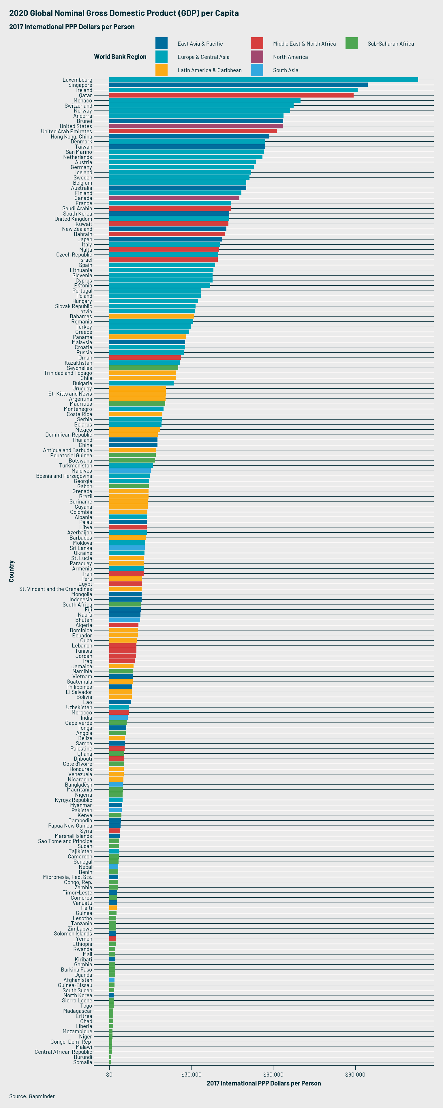
current_gdp <- clean_ts_data %>%
  filter(year == 2020) %>%
  filter(!is.na(region_wb)) %>%
  arrange(gdp_per_capita_est) %>%
  mutate(country = factor(country,ordered=TRUE,levels = unique(country))) %>%
  filter(!is.na(gdp_per_capita_est))

ggplot(current_gdp,aes(x=country,y=gdp_per_capita_est,fill=region_wb))+
  geom_col()+
  coord_flip()+
  scale_fill_manual(values = nn_base_color_palette %>%
                      filter(color_category != "Background") %>%
                      pull(hex_code),
                    name="World Bank Region")+
  nn_basic_theme(base_size = 18) +
  scale_y_continuous(labels = dollar)+
  labs(title = "2020 Global Nominal Gross Domestic Product (GDP) per Capita",
       subtitle = "2017 International PPP Dollars per Person",
       caption = "Source: Gapminder",
       y="2017 International PPP Dollars per Person",
       x="Country")+
  guides(fill = guide_legend(nrow=3))
Maps
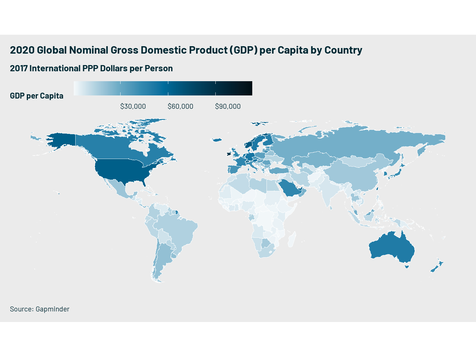
current_gdp_map <- current_gdp %>%
  left_join(world_countries %>%
              select(iso_n3,geometry)) %>%
  st_as_sf()

ggplot()+
  geom_sf(data =current_gdp_map,aes(fill=gdp_per_capita_est),size=0.01,color="white")+
  coord_sf()+
  nn_basic_theme(base_size=22)+
  scale_fill_gradientn(colors= nn_color_ramp(num_colors = 9,palette_name = "Blue"),
                        labels=dollar, name="GDP per Capita")+
  labs(title = "2020 Global Nominal Gross Domestic Product (GDP) per Capita by Country",
       subtitle = "2017 International PPP Dollars per Person",
       caption = "Source: Gapminder")+
  theme(legend.key.width = unit(3,"lines"),
        axis.line.x = element_blank(),
        axis.text.x = element_blank(),
        axis.ticks = element_blank())
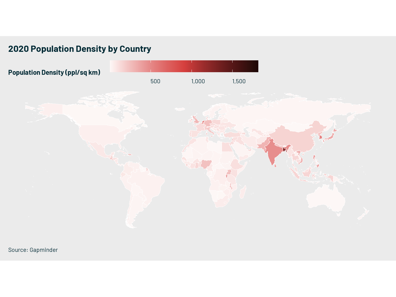
ggplot()+
  geom_sf(data =current_gdp_map %>% filter(pop_density <=2000),
          aes(fill=pop_density),size=0.01,color="white")+
  coord_sf()+
  nn_basic_theme(base_size=22)+
  scale_fill_gradientn(colors= nn_color_ramp(num_colors = 9,palette_name = "Red"),
                        labels=comma, name="Population Density (ppl/sq km)")+
  labs(title = "2020 Population Density by Country",
       caption = "Source: Gapminder")+
  theme(legend.key.width = unit(3,"lines"),
        axis.line.x = element_blank(),
        axis.text.x = element_blank(),
        axis.ticks = element_blank())
Scatter Plot
current_gdp_density <- clean_ts_data %>%
filter(year == 2020) %>%
filter(!is.na(region_wb))
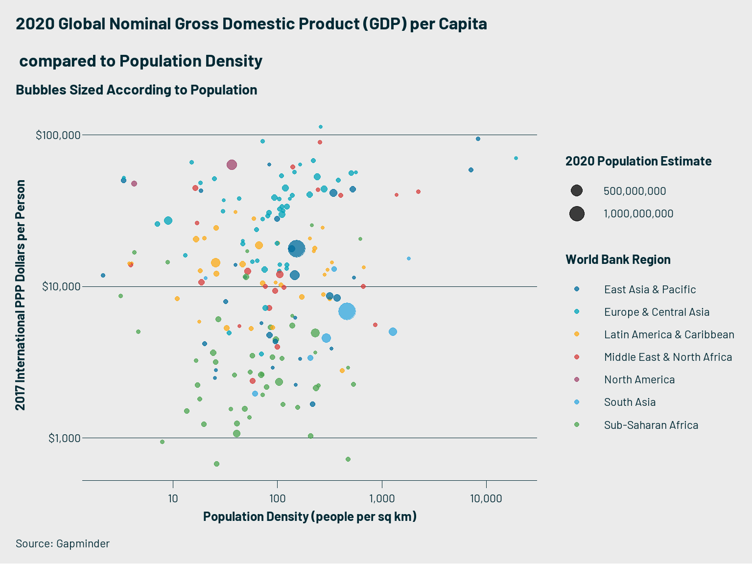
ggplot(current_gdp_density,
aes(x = pop_density,y=gdp_per_capita_est,size=pop_est,
color=region_wb))+
geom_point(alpha=0.75) +
scale_x_log10(labels=comma) +
scale_y_log10(labels=dollar)+
nn_basic_theme(legend_right = TRUE,base_size=22)+
scale_size_continuous(labels=comma, name="2020 Population Estimate")+
scale_color_manual(values = nn_base_color_palette %>%
filter(color_category != "Background") %>%
pull(hex_code),
name="World Bank Region")+
labs(
title = "2020 Global Nominal Gross Domestic Product (GDP) per Capita\n compared to Population Density",
subtitle = "Bubbles Sized According to Population",
caption = "Source: Gapminder",
y="2017 International PPP Dollars per Person",
x="Population Density (people per sq km)"
)