This content was presented to Nelson\Nygaard Staff at a Lunch and Learn webinar on Thursday, August 5th 2021, and is available as a recording here and embedded below.
Today’s Agenda
- R markdown basics (45 minutes)
- Loading example HTML output onto GitHub pages (15 minutes)
R Markdown Basics
Introduction
R Markdown provides an unified authoring framework for data science, combining your code, its results, and your prose commentary. R Markdown documents are fully reproducible and support dozens of output formats, like PDFs, Word files, slideshows, and more.
R Markdown files are designed to be used in three ways:
For communicating to decision makers, who want to focus on the conclusions, not the code behind the analysis.
For collaborating with other data scientists (including future you!), who are interested in both your conclusions, and how you reached them (i.e. the code).
As an environment in which to do data science, as a modern day lab notebook where you can capture not only what you did, but also what you were thinking.
R Markdown integrates a number of R packages and external tools. This means that help is, by-and-large, not available through ?. Instead, as you work through this chapter, and use R Markdown in the future, keep these resources close to hand:
R Markdown Cheat Sheet: Help > Cheatsheets > R Markdown Cheat Sheet,
R Markdown Reference Guide: Help > Cheatsheets > R Markdown Reference Guide.
Both cheatsheets are also available at http://rstudio.com/cheatsheets.
Prerequisites
You need the rmarkdown package, but you don’t need to explicitly install it or load it, as RStudio automatically does both when needed.
R Markdown basics
This is an R Markdown file, a plain text file that has the extension .Rmd:
---
title: "Diamond sizes"
date: 2016-08-25
output: html_document
---
```{r setup, include = FALSE}
library(ggplot2)
library(dplyr)
smaller <- diamonds %>%
filter(carat <= 2.5)
```
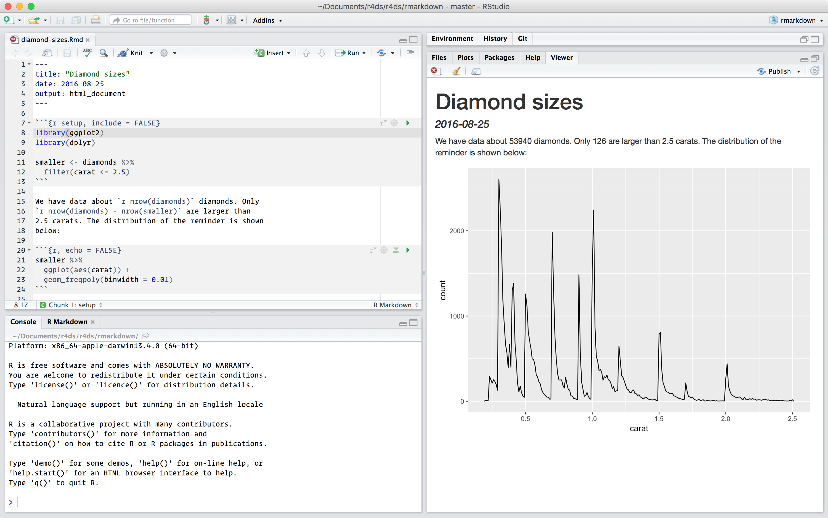
We have data about `r nrow(diamonds)` diamonds. Only
`r nrow(diamonds) - nrow(smaller)` are larger than
2.5 carats. The distribution of the remainder is shown
below:
```{r, echo = FALSE}
smaller %>%
ggplot(aes(carat)) +
geom_freqpoly(binwidth = 0.01)
```It contains three important types of content:
- An (optional) YAML header surrounded by
---s. - Chunks of R code surrounded by
```. - Text mixed with simple text formatting like
# headingand_italics_.
When you open an .Rmd, you get a notebook interface where code and output are interleaved. You can run each code chunk by clicking the Run icon (it looks like a play button at the top of the chunk), or by pressing Cmd/Ctrl + Shift + Enter. RStudio executes the code and displays the results inline with the code:

To produce a complete report containing all text, code, and results, click “Knit” or press Cmd/Ctrl + Shift + K. You can also do this programmatically with rmarkdown::render("1-example.Rmd"). This will display the report in the viewer pane, and create a self-contained HTML file that you can share with others.
When you knit the document, R Markdown sends the .Rmd file to knitr, http://yihui.name/knitr/, which executes all of the code chunks and creates a new markdown (.md) document which includes the code and its output. The markdown file generated by knitr is then processed by pandoc, http://pandoc.org/, which is responsible for creating the finished file. The advantage of this two step workflow is that you can create a very wide range of output formats, as you’ll learn about in [R markdown formats].

To get started with your own .Rmd file, select File > New File > R Markdown… in the menubar. RStudio will launch a wizard that you can use to pre-populate your file with useful content that reminds you how the key features of R Markdown work.
The following sections dive into the three components of an R Markdown document in more details: the markdown text, the code chunks, and the YAML header.
Text formatting with Markdown
Prose in .Rmd files is written in Markdown, a lightweight set of conventions for formatting plain text files. Markdown is designed to be easy to read and easy to write. It is also very easy to learn. The guide below shows how to use Pandoc’s Markdown, a slightly extended version of Markdown that R Markdown understands.
Text formatting
------------------------------------------------------------
*italic* or _italic_
**bold** __bold__
`code`
superscript^2^ and subscript~2~
Headings
------------------------------------------------------------
# 1st Level Header
## 2nd Level Header
### 3rd Level Header
Lists
------------------------------------------------------------
* Bulleted list item 1
* Item 2
* Item 2a
* Item 2b
1. Numbered list item 1
1. Item 2. The numbers are incremented automatically in the output.
Links and images
------------------------------------------------------------
<http://example.com>
[linked phrase](http://example.com)

Tables
------------------------------------------------------------
First Header | Second Header
------------- | -------------
Content Cell | Content Cell
Content Cell | Content CellThe best way to learn these is simply to try them out. It will take a few days, but soon they will become second nature, and you won’t need to think about them. If you forget, you can get to a handy reference sheet with Help > Markdown Quick Reference.
Code chunks
To run code inside an R Markdown document, you need to insert a chunk. There are three ways to do so:
The keyboard shortcut Cmd/Ctrl + Alt + I
The “Insert” button icon in the editor toolbar.
By manually typing the chunk delimiters
```{r}and```.
Obviously, I’d recommend you learn the keyboard shortcut. It will save you a lot of time in the long run!
You can continue to run the code using the keyboard shortcut that by now (I hope!) you know and love: Cmd/Ctrl + Enter. However, chunks get a new keyboard shortcut: Cmd/Ctrl + Shift + Enter, which runs all the code in the chunk. Think of a chunk like a function. A chunk should be relatively self-contained, and focused around a single task.
The following sections describe the chunk header which consists of ```{r, followed by an optional chunk name, followed by comma separated options, followed by }. Next comes your R code and the chunk end is indicated by a final ```.
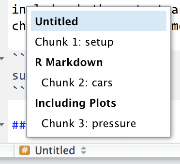
Chunk name
Chunks can be given an optional name: ```{r by-name}. This has three advantages:
You can more easily navigate to specific chunks using the drop-down code navigator in the bottom-left of the script editor:
Graphics produced by the chunks will have useful names that make them easier to use elsewhere. More on that in [other important options].
You can set up networks of cached chunks to avoid re-performing expensive computations on every run. More on that below.
There is one chunk name that imbues special behavior: setup. When you’re in a notebook mode, the chunk named setup will be run automatically once, before any other code is run.
Chunk options
Chunk output can be customized with options, arguments supplied to chunk header. Knitr provides almost 60 options that you can use to customize your code chunks. Here we’ll cover the most important chunk options that you’ll use frequently. You can see the full list at http://yihui.name/knitr/options/.
The most important set of options controls if your code block is executed and what results are inserted in the finished report:
eval = FALSEprevents code from being evaluated. (And obviously if the code is not run, no results will be generated). This is useful for displaying example code, or for disabling a large block of code without commenting each line.include = FALSEruns the code, but doesn’t show the code or results in the final document. Use this for setup code that you don’t want cluttering your report.echo = FALSEprevents code, but not the results from appearing in the finished file. Use this when writing reports aimed at people who don’t want to see the underlying R code.message = FALSEorwarning = FALSEprevents messages or warnings from appearing in the finished file.results = 'hide'hides printed output;fig.show = 'hide'hides plots.error = TRUEcauses the render to continue even if code returns an error. This is rarely something you’ll want to include in the final version of your report, but can be very useful if you need to debug exactly what is going on inside your.Rmd. It’s also useful if you’re teaching R and want to deliberately include an error. The default,error = FALSEcauses knitting to fail if there is a single error in the document.
The following table summarises which types of output each option supressess:
| Option | Run code | Show code | Output | Plots | Messages | Warnings |
|---|---|---|---|---|---|---|
eval = FALSE |
- | - | - | - | - | |
include = FALSE |
- | - | - | - | - | |
echo = FALSE |
- | |||||
results = "hide" |
- | |||||
fig.show = "hide" |
- | |||||
message = FALSE |
- | |||||
warning = FALSE |
- |
Table
By default, R Markdown prints data frames and matrices as you’d see them in the console:
mtcars[1:5, ]
                   mpg cyl disp  hp drat    wt  qsec vs am gear carb
Mazda RX4         21.0   6  160 110 3.90 2.620 16.46  0  1    4    4
Mazda RX4 Wag     21.0   6  160 110 3.90 2.875 17.02  0  1    4    4
Datsun 710        22.8   4  108  93 3.85 2.320 18.61  1  1    4    1
Hornet 4 Drive    21.4   6  258 110 3.08 3.215 19.44  1  0    3    1
Hornet Sportabout 18.7   8  360 175 3.15 3.440 17.02  0  0    3    2
If you prefer that data be displayed with additional formatting you can use the knitr::kable function. The code below generates Table 1.
knitr::kable(
  mtcars[1:5, ],
  caption = "A knitr kable."
)
| mpg | cyl | disp | hp | drat | wt | qsec | vs | am | gear | carb | |
|---|---|---|---|---|---|---|---|---|---|---|---|
| Mazda RX4 | 21.0 | 6 | 160 | 110 | 3.90 | 2.620 | 16.46 | 0 | 1 | 4 | 4 |
| Mazda RX4 Wag | 21.0 | 6 | 160 | 110 | 3.90 | 2.875 | 17.02 | 0 | 1 | 4 | 4 |
| Datsun 710 | 22.8 | 4 | 108 | 93 | 3.85 | 2.320 | 18.61 | 1 | 1 | 4 | 1 |
| Hornet 4 Drive | 21.4 | 6 | 258 | 110 | 3.08 | 3.215 | 19.44 | 1 | 0 | 3 | 1 |
| Hornet Sportabout | 18.7 | 8 | 360 | 175 | 3.15 | 3.440 | 17.02 | 0 | 0 | 3 | 2 |
Read the documentation for ?knitr::kable to see the other ways in which you can customize the table. For even deeper customization, consider the DT, xtable, stargazer, pander, tables, and ascii packages. Each provides a set of tools for returning formatted tables from R code.
There is also a rich set of options for controlling how figures are embedded. You’ll learn about these in [saving your plots].
Caching
Normally, each knit of a document starts from a completely clean slate. This is great for reproducibility, because it ensures that you’ve captured every important computation in code. However, it can be painful if you have some computations that take a long time. The solution is cache = TRUE. When set, this will save the output of the chunk to a specially named file on disk. On subsequent runs, knitr will check to see if the code has changed, and if it hasn’t, it will reuse the cached results.
The caching system must be used with care, because by default it is based on the code only, not its dependencies. For example, here the processed_data chunk depends on the raw_data chunk:
```{r raw_data}
rawdata <- readr::read_csv("a_very_large_file.csv")
```

```{r processed_data, cache = TRUE}
processed_data <- rawdata %>%
  filter(!is.na(import_var)) %>%
  mutate(new_variable = complicated_transformation(x, y, z))
```
Caching the processed_data chunk means that it will get re-run if the dplyr pipeline is changed, but it won’t get rerun if the read_csv() call changes. You can avoid that problem with the dependson chunk option:
```{r processed_data, cache = TRUE, dependson = "raw_data"}
processed_data <- rawdata %>%
  filter(!is.na(import_var)) %>%
  mutate(new_variable = complicated_transformation(x, y, z))
```
dependson should contain a character vector of every chunk that the cached chunk depends on. Knitr will update the results for the cached chunk whenever it detects that one of its dependencies have changed.
Note that the chunks won’t update if a_very_large_file.csv changes, because knitr caching only tracks changes within the .Rmd file. If you want to also track changes to that file you can use the cache.extra option. This is an arbitrary R expression that will invalidate the cache whenever it changes. A good function to use is file.info(): it returns a bunch of information about the file including when it was last modified. Then you can write:
```{r raw_data, cache.extra = file.info("a_very_large_file.csv")}
rawdata <- readr::read_csv("a_very_large_file.csv")
```
As your caching strategies get progressively more complicated, it’s a good idea to regularly clear out all your caches with knitr::clean_cache().
I’ve used the advice of David Robinson to name these chunks: each chunk is named after the primary object that it creates. This makes it easier to understand the dependson specification.
Global options
As you work more with knitr, you will discover that some of the default chunk options don’t fit your needs and you want to change them. You can do this by calling knitr::opts_chunk$set() in a code chunk. For example, when writing books and tutorials I set:
knitr::opts_chunk$set(
  comment = "#>",
  collapse = TRUE
)
This uses my preferred comment formatting, and ensures that the code and output are kept closely entwined. On the other hand, if you were preparing a report, you might set:
knitr::opts_chunk$set(
  echo = FALSE
)
That will hide the code by default, so only showing the chunks you deliberately choose to show (with echo = TRUE). You might consider setting message = FALSE and warning = FALSE, but that would make it harder to debug problems because you wouldn’t see any messages in the final document.
Inline code
There is one other way to embed R code into an R Markdown document: directly into the text, with: `r `. This can be very useful if you mention properties of your data in the text. For example, in the example document I used at the start of the chapter I had:
We have data about
`r nrow(diamonds)`diamonds. Only`r nrow(diamonds) - nrow(smaller)`are larger than 2.5 carats. The distribution of the remainder is shown below:
When the report is knit, the results of these computations are inserted into the text:
We have data about 53940 diamonds. Only 126 are larger than 2.5 carats. The distribution of the remainder is shown below:
When inserting numbers into text, format() is your friend. It allows you to set the number of digits so you don’t print to a ridiculous degree of accuracy, and a big.mark to make numbers easier to read. I’ll often combine these into a helper function:
comma <- function(x) format(x, digits = 2, big.mark = ",")
comma(3452345)
[1] "3,452,345"comma(.12358124331)
[1] "0.12"Troubleshooting
Troubleshooting R Markdown documents can be challenging because you are no longer in an interactive R environment, and you will need to learn some new tricks. The first thing you should always try is to recreate the problem in an interactive session. Restart R, then “Run all chunks” (either from Code menu, under Run region), or with the keyboard shortcut Ctrl + Alt + R. If you’re lucky, that will recreate the problem, and you can figure out what’s going on interactively.
If that doesn’t help, there must be something different between your interactive environment and the R markdown environment. You’re going to need to systematically explore the options. The most common difference is the working directory: the working directory of an R Markdown is the directory in which it lives. Check the working directory is what you expect by including getwd() in a chunk.
Next, brainstorm all the things that might cause the bug. You’ll need to systematically check that they’re the same in your R session and your R markdown session. The easiest way to do that is to set error = TRUE on the chunk causing the problem, then use print() and str() to check that settings are as you expect.
YAML header
You can control many other “whole document” settings by tweaking the parameters of the YAML header. You might wonder what YAML stands for: it’s “yet another markup language”, which is designed for representing hierarchical data in a way that’s easy for humans to read and write. R Markdown uses it to control many details of the output. Here we’ll discuss two: document parameters and bibliographies.
Parameters
R Markdown documents can include one or more parameters whose values can be set when you render the report. Parameters are useful when you want to re-render the same report with distinct values for various key inputs. For example, you might be producing sales reports per branch, exam results by student, or demographic summaries by country. To declare one or more parameters, use the params field.
This example uses a my_class parameter to determine which class of cars to display:
---
output: html_document
params:
  my_class: "suv"
---

```{r setup, include = FALSE}
library(ggplot2)
library(dplyr)

class <- mpg %>% filter(class == params$my_class)
```

# Fuel economy for `r params$my_class`s

```{r, message = FALSE}
ggplot(class, aes(displ, hwy)) +
  geom_point() +
  geom_smooth(se = FALSE)
```
As you can see, parameters are available within the code chunks as a read-only list named params.
You can write atomic vectors directly into the YAML header. You can also run arbitrary R expressions by prefacing the parameter value with !r. This is a good way to specify date/time parameters.
params:
  start: !r lubridate::ymd("2015-01-01")
  snapshot: !r lubridate::ymd_hms("2015-01-01 12:30:00")
In RStudio, you can click the “Knit with Parameters” option in the Knit dropdown menu to set parameters, render, and preview the report in a single user friendly step. You can customize the dialog by setting other options in the header. See http://rmarkdown.rstudio.com/developer_parameterized_reports.html#parameter_user_interfaces for more details.
Alternatively, if you need to produce many such paramterised reports, you can call rmarkdown::render() with a list of params:
This is particularly powerful in conjunction with purrr:pwalk(). The following example creates a report for each value of class found in mpg. First we create a data frame that has one row for each class, giving the filename of the report and the params:
reports <- tibble(
  class = unique(mpg$class),
  filename = stringr::str_c("fuel-economy-", class, ".html"),
  params = purrr::map(class, ~ list(my_class = .))
)
reports
# A tibble: 7 x 3
  class      filename                     params
  <chr>      <chr>                        <list>
1 compact    fuel-economy-compact.html    <named list [1]>
2 midsize    fuel-economy-midsize.html    <named list [1]>
3 suv        fuel-economy-suv.html        <named list [1]>
4 2seater    fuel-economy-2seater.html    <named list [1]>
5 minivan    fuel-economy-minivan.html    <named list [1]>
6 pickup     fuel-economy-pickup.html     <named list [1]>
7 subcompact fuel-economy-subcompact.html <named list [1]>
Then we match the column names to the argument names of render(), and use purrr’s parallel walk to call render() once for each row:
Visual R Markdown Editor
Overview
Now that you know the basics of R markdown, I can show you a new tool that could potentially make usage easier – RStudio v1.4 includes a new visual markdown editing mode! Highlights of visual mode include:
Visual editing for all of Pandoc markdown, including tables, divs/spans, definition lists, attributes, etc.
Extensive support for citations
Scientific and technical writing features, including cross-references, footnotes, equations, code execution, and embedded LaTeX.
Writing productivity features, including real time spell-checking and outline navigation.
Tight integration with source editing (editing location and undo/redo state are preserved when switching between modes).
Rich keyboard support. In addition to traditional shortcuts, you can use markdown expressions (e.g.
##,**bold**, etc.) for formatting. If you don’t remember all of the keyboard shortcuts, you can also use the catch-all ⌃ / shortcut to insert anything.
Getting Started
Visual markdown editing is available in RStudio v1.4 or higher. You can download the latest version of RStudio here: https://rstudio.com/products/rstudio/download/.
Markdown documents can be edited in either source or visual mode. To switch into visual mode for a given document, use the compass button at the top-right of the document toolbar (or alternatively the ⌃⇧ F4 keyboard shortcut):
Note that you can switch between source and visual mode at any time (editing location and undo/redo state will be preserved when you switch).
Using the Editor
Keyboard Shortcuts
There are keyboard shortcuts for all basic editing tasks. Visual mode supports both traditional keyboard shortcuts (e.g. ⌃ B for bold) as well as markdown shortcuts (using markdown syntax directly). For example, enclose **bold** text in asterisks or type ## and press space to create a second level heading. Here are some of the most commonly used shortcuts:
| Command | Keyboard Shortcut | Markdown Shortcut |
|---|---|---|
| Bold | ⌃ B | **bold** |
| Italic | ⌃ I | *italic* |
| Code | ⌃ D | `code` |
| Link | ⌃ K | <href> |
| Heading 1 | ⌥⌃ 1 | # |
| Heading 2 | ⌥⌃ 2 | ## |
| Heading 3 | ⌥⌃ 3 | ### |
| R Code Chunk | ⌥⌃ I | ```{r} |
See the editing shortcuts article for a complete list of all shortcuts.
Insert Anything
You can also use the catch-all ⌃ / shortcut to insert just about anything. Just execute the shortcut then type what you want to insert. For example:
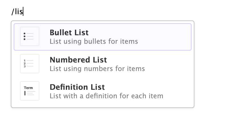
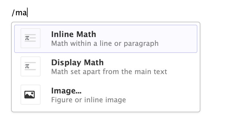
If you are at the beginning of a line (as displayed above), you can also enter plain / to invoke the shortcut.
Editor Toolbar
The editor toolbar includes buttons for the most commonly used formatting commands:

Additional commands are available on the Format, Insert, and Table menus:
| Format | Insert | Table |
|---|---|---|
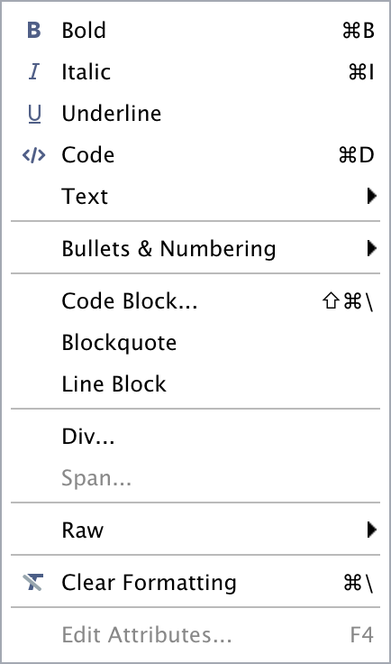 |
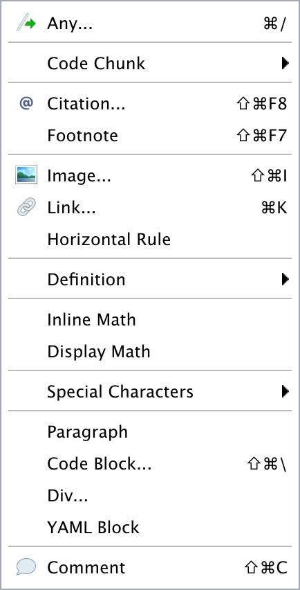 |
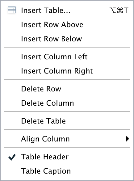 |
More About Visual Editing
Check out the following articles to learn more about visual markdown editing:
Citations covers citing other works and managing bibliographies, as well as integration with Zotero (an open source reference management tool).
Technical Writing covers features commonly used in scientific and technical writing, including cross-references, footnotes, equations, embedded code, and LaTeX.
Content Editing provides more depth on visual editor support for tables, lists, pandoc attributes, comments, symbols/emojis, etc.
Markdown Formats describes how the visual editor parses and writes markdown, and also includes some tips for usage with Bookdown and Hugo.
Editing Shortcuts documents the two types of shortcuts you can use with the editor: standard keyboard shortcuts and markdown shortcuts.
Editor Options enumerates the various ways you can configure the behavior of the editor (font size, display width, markdown output, etc.).
Additional Topics discusses various other features including using CSS within HTML documents.
GitHub Pages Example
I’m going to show you basics of publishing an HTML page to GitHub Pages. It is very easy to do and the example we are going to use is only a single HTML file, but you can nest as many as you want in directory structure – this training website itself is built in markdown and published using GitHub pages.
I have set up a very simple GitHub pages example here.
Initial steps
First, you’ll want to create an R project to house your code, data, and the web page(s). If you already have an existing R Project, make a
docsfolder within the main directory. This will come up later.Next, you will want to set up version control using git in your R project. This can be done within RStudio in Tools > Version Control > Project Setup. If this is already done, move to the next step.
In the folder where your website lives, you will want to create an
index.Rmdfile (which will be knit to anindex.htmlfile) to be the index for your website – this is what will come up to the user when the base directory of the website is visited. Link to your other pages from here as needed.You will want to commit and push your local repository to the remote repository on GitHub. See our previous GitHub trainings if you are unsure about how to do this.
Settings in GitHub
- Within GitHub, you will want to navigate to your repository. Then you will want to go to Settings > Pages – this is where you can access all settings for GitHub Pages.
- Then, you will want to change ‘None’, to the branch on which your GitHub Pages website lives. Most of the time, this will be main (or master). You will then want to set the base directory of your website to either
/rootor/docs(this is why we may have created the/docsfolder earlier. This depends on whether the sole function of the repository is to be a website, or if the website is an ancillary piece to the repository (like documentation). Then click ‘Save’. - Once you do that, you will receive a notice of your website’s address. Sometimes the website itself will take a few minutes to publish, so if it is not available immediately, check back in 5-10 minutes.
- That’s it! You can see our very simple web page here. This is a very easy way to share R code/content/narrative with a client, and can be customized endlessly. I will leave a few resources below for customization.
Learning more
R Markdown is still relatively young, and is still growing rapidly. The best place to stay on top of innovations is the official R Markdown website: <http://rmarkdown.rstudio.com>.
The best R Markdown book out there to date is R Markdown: The Definitive Guide, available for free online.
R Markdown can be styled in many ways. Some of my favorites are:
bookdownis a package for outputting a set of markdown pages in a book-like structure. The above book (and indeed many online R books) are knitted usingbookdown. A full reference book (of course, written inbookdown!) on usingbookdownis available here.distillis a package for knitting a web publishing format optimized for scientific and technical communication. The NN R Training website is knitted into adistillblog. Documentation is here.A bunch of other formats, including your MS Office favorites like Word and Powerpoint, are described in the above referenced book.
This content was presented to Nelson\Nygaard Staff at a Lunch and Learn webinar on Thursday, August 5th 2021, and is available as a recording here and embedded above.