This content was presented to Nelson\Nygaard Staff at a Lunch and Learn webinar on Wednesday, February 17th, 2021, and is available as a recording here and embedded below.
Today’s Agenda
Acknowledgement: This module heavily draws upon Hadley Wickham’s (the progenitor of the Tidyverse) book (available for free online), R for Data Science, including text, pictures, and code directly copied from that book and slightly modified to suit a shorter narrative. Printed copies are available generally wherever you get your books. It is recommended that you read this book for a deeper understanding of the topics contained hereien – only basic concepts are able to be covered within the time available.
Functions
Introduction
One of the best ways to improve your reach as a data scientist is to write functions. Functions allow you to automate common tasks in a more powerful and general way than copy-and-pasting. Writing a function has three big advantages over using copy-and-paste:
You can give a function an evocative name that makes your code easier to understand.
As requirements change, you only need to update code in one place, instead of many.
You eliminate the chance of making incidental mistakes when you copy and paste (i.e. updating a variable name in one place, but not in another).
Writing good functions is a lifetime journey. Even after using R for many years, I still learn new techniques and better ways of approaching old problems. The goal of this section is not to teach you every esoteric detail of functions but to get you started with some pragmatic advice that you can apply immediately.
As well as practical advice for writing functions, this section also gives you some suggestions for how to style your code. Good code style is like correct punctuation. Youcanmanagewithoutit, but it sure makes things easier to read! As with styles of punctuation, there are many possible variations. Here we present the style we use in our code, but the most important thing is to be consistent.
When should you write a function?
You should consider writing a function whenever you’ve copied and pasted a block of code more than twice (i.e., you now have three copies of the same code). For example, take a look at this code. What does it do?
library(tidyverse)
df <- tibble::tibble(
  a = rnorm(10),
  b = rnorm(10),
  c = rnorm(10),
  d = rnorm(10)
)

df$a <- (df$a - min(df$a, na.rm = TRUE)) /
  (max(df$a, na.rm = TRUE) - min(df$a, na.rm = TRUE))
df$b <- (df$b - min(df$b, na.rm = TRUE)) /
  (max(df$b, na.rm = TRUE) - min(df$a, na.rm = TRUE))
df$c <- (df$c - min(df$c, na.rm = TRUE)) /
  (max(df$c, na.rm = TRUE) - min(df$c, na.rm = TRUE))
df$d <- (df$d - min(df$d, na.rm = TRUE)) /
  (max(df$d, na.rm = TRUE) - min(df$d, na.rm = TRUE))
You might be able to puzzle out that this rescales each column to have a range from 0 to 1. But did you spot the mistake? I made an error when copying-and-pasting the code for df$b: I forgot to change an a to a b. Extracting repeated code out into a function is a good idea because it prevents you from making this type of mistake.
To write a function you need to first analyze the code. How many inputs does it have?
This code only has one input: df$a. (If you’re surprised that TRUE is not an input, you can explore why in the exercise below.) To make the inputs more clear, it’s a good idea to rewrite the code using temporary variables with general names. Here this code only requires a single numeric vector, so I’ll call it x:
 [1] 0.0000000 1.0000000 0.2954605 0.7061987 0.7293579 0.5586090
 [7] 0.2478625 0.5198846 0.8565695 0.6071605
There is some duplication in this code. We’re computing the range of the data three times, so it makes sense to do it in one step:
rng <- range(x, na.rm = TRUE)
(x - rng[1]) / (rng[2] - rng[1])
 [1] 0.0000000 1.0000000 0.2954605 0.7061987 0.7293579 0.5586090
 [7] 0.2478625 0.5198846 0.8565695 0.6071605
Pulling out intermediate calculations into named variables is a good practice because it makes it more clear what the code is doing. Now that I’ve simplified the code, and checked that it still works, I can turn it into a function:
rescale01 <- function(x) {
  rng <- range(x, na.rm = TRUE)
  (x - rng[1]) / (rng[2] - rng[1])
}
rescale01(c(0, 5, 10))
[1] 0.0 0.5 1.0There are three key steps to creating a new function:
You need to pick a name for the function. Here I’ve used
rescale01because this function rescales a vector to lie between 0 and 1.You list the inputs, or arguments, to the function inside
function. Here we have just one argument. If we had more the call would look likefunction(x, y, z).You place the code you have developed in body of the function, a
{block that immediately followsfunction(...).
Note the overall process: I only made the function after I’d figured out how to make it work with a simple input. It’s easier to start with working code and turn it into a function; it’s harder to create a function and then try to make it work.
At this point it’s a good idea to check your function with a few different inputs:
As you write more and more functions you’ll eventually want to convert these informal, interactive tests into formal, automated tests. That process is called unit testing. Unfortunately, it’s beyond the scope of this module, but you can learn about it in http://r-pkgs.had.co.nz/tests.html.
We can simplify the original example now that we have a function:
df$a <- rescale01(df$a)
df$b <- rescale01(df$b)
df$c <- rescale01(df$c)
df$d <- rescale01(df$d)
Compared to the original, this code is easier to understand and we’ve eliminated one class of copy-and-paste errors. There is still quite a bit of duplication since we’re doing the same thing to multiple columns. We’ll learn how to eliminate that duplication in iteration, once you’ve learned more about R’s data structures in [vectors].
Another advantage of functions is that if our requirements change, we only need to make the change in one place. For example, we might discover that some of our variables include infinite values, and rescale01() fails:
x <- c(1:10, Inf)
rescale01(x)
[1] 0 0 0 0 0 0 0 0 0 0 NaNBecause we’ve extracted the code into a function, we only need to make the fix in one place:
rescale01 <- function(x) {
  rng <- range(x, na.rm = TRUE, finite = TRUE)
  (x - rng[1]) / (rng[2] - rng[1])
}
rescale01(x)
 [1] 0.0000000 0.1111111 0.2222222 0.3333333 0.4444444 0.5555556
 [7] 0.6666667 0.7777778 0.8888889 1.0000000       Inf
Functions are for humans and computers
It’s important to remember that functions are not just for the computer, but are also for humans. R doesn’t care what your function is called, or what comments it contains, but these are important for human readers. This section discusses some things that you should bear in mind when writing functions that humans can understand.
The name of a function is important. Ideally, the name of your function will be short, but clearly evoke what the function does. That’s hard! But it’s better to be clear than short, as RStudio’s auto-complete makes it easy to type long names.
Generally, function names should be verbs, and arguments should be nouns. There are some exceptions: nouns are OK if the function computes a very well known noun (i.e. mean() is better than compute_mean()), or accessing some property of an object (i.e. coef() is better than get_coefficients()). A good sign that a noun might be a better choice is if you’re using a very broad verb like “get”, “compute”, “calculate”, or “determine”. Use your best judgment and don’t be afraid to rename a function if you figure out a better name later.
# Too short
f()

# Not a verb, or descriptive
my_awesome_function()

# Long, but clear
impute_missing()
collapse_years()
If your function name is composed of multiple words, I recommend using “snake_case”, where each lowercase word is separated by an underscore. camelCase is a popular alternative. It doesn’t really matter which one you pick, the important thing is to be consistent: pick one or the other and stick with it. R itself is not very consistent, but there’s nothing you can do about that. Make sure you don’t fall into the same trap by making your code as consistent as possible.
# Never do this!
col_mins <- function(x, y) {}
rowMaxes <- function(y, x) {}
If you have a family of functions that do similar things, make sure they have consistent names and arguments. Use a common prefix to indicate that they are connected. That’s better than a common suffix because auto-complete allows you to type the prefix and see all the members of the family.
# Good
input_select()
input_checkbox()
input_text()

# Not so good
select_input()
checkbox_input()
text_input()
A good example of this design is the stringr package: if you don’t remember exactly which function you need, you can type str_ and jog your memory.
Where possible, avoid overriding existing functions and variables. It’s impossible to do in general because so many good names are already taken by other packages, but avoiding the most common names from base R will avoid confusion.
# Don't do this!
T <- FALSE
c <- 10
mean <- function(x) sum(x)
Use comments, lines starting with #, to explain the “why” of your code. You generally should avoid comments that explain the “what” or the “how”. If you can’t understand what the code does from reading it, you should think about how to rewrite it to be more clear. Do you need to add some intermediate variables with useful names? Do you need to break out a subcomponent of a large function so you can name it? However, your code can never capture the reasoning behind your decisions: why did you choose this approach instead of an alternative? What else did you try that didn’t work? It’s a great idea to capture that sort of thinking in a comment.
Another important use of comments is to break up your file into easily readable chunks. Use long lines of - and = to make it easy to spot the breaks.
# Load data --------------------------------------

# Plot data --------------------------------------
Function arguments
The arguments to a function typically fall into two broad sets: one set supplies the data to compute on, and the other supplies arguments that control the details of the computation. For example:
In
log(), the data isx, and the detail is thebaseof the logarithm.In
mean(), the data isx, and the details are how much data to trim from the ends (trim) and how to handle missing values (na.rm).In
t.test(), the data arexandy, and the details of the test arealternative,mu,paired,var.equal, andconf.level.In
str_c()you can supply any number of strings to..., and the details of the concatenation are controlled bysepandcollapse.
Generally, data arguments should come first. Detail arguments should go on the end, and usually should have default values. You specify a default value in the same way you call a function with a named argument:
# Compute confidence interval around mean using normal approximation
mean_ci <- function(x, conf = 0.95) {
  se <- sd(x) / sqrt(length(x))
  alpha <- 1 - conf
  mean(x) + se * qnorm(c(alpha / 2, 1 - alpha / 2))
}

x <- runif(100)
mean_ci(x)
[1] 0.4608990 0.5700401mean_ci(x, conf = 0.99)
[1] 0.4437517 0.5871874The default value should almost always be the most common value. The few exceptions to this rule are to do with safety. For example, it makes sense for na.rm to default to FALSE because missing values are important. Even though na.rm = TRUE is what you usually put in your code, it’s a bad idea to silently ignore missing values by default.
When you call a function, you typically omit the names of the data arguments, because they are used so commonly. If you override the default value of a detail argument, you should use the full name:
You can refer to an argument by its unique prefix (e.g. mean(x, n = TRUE)), but this is generally best avoided given the possibilities for confusion.
Notice that when you call a function, you should place a space around = in function calls, and always put a space after a comma, not before (just like in regular English). Using whitespace makes it easier to skim the function for the important components.
Choosing names
The names of the arguments are also important. R doesn’t care, but the readers of your code (including future-you!) will. Generally you should prefer longer, more descriptive names, but there are a handful of very common, very short names. It’s worth memorising these:
x,y,z: vectors.w: a vector of weights.df: a data frame.i,j: numeric indices (typically rows and columns).n: length, or number of rows.p: number of columns.
Otherwise, consider matching names of arguments in existing R functions. For example, use na.rm to determine if missing values should be removed.
Checking values
As you start to write more functions, you’ll eventually get to the point where you don’t remember exactly how your function works. At this point it’s easy to call your function with invalid inputs. To avoid this problem, it’s often useful to make constraints explicit. For example, imagine you’ve written some functions for computing weighted summary statistics:
What happens if x and w are not the same length?
wt_mean(1:6, 1:3)
[1] 7.666667In this case, because of R’s vector recycling rules, we don’t get an error.
It’s good practice to check important preconditions, and throw an error (with stop()), if they are not true:
Be careful not to take this too far. There’s a tradeoff between how much time you spend making your function robust, versus how long you spend writing it. For example, if you also added a na.rm argument, I probably wouldn’t check it carefully:
wt_mean <- function(x, w, na.rm = FALSE) {
  if (!is.logical(na.rm)) {
    stop("`na.rm` must be logical")
  }
  if (length(na.rm) != 1) {
    stop("`na.rm` must be length 1")
  }
  if (length(x) != length(w)) {
    stop("`x` and `w` must be the same length", call. = FALSE)
  }

  if (na.rm) {
    miss <- is.na(x) | is.na(w)
    x <- x[!miss]
    w <- w[!miss]
  }
  sum(w * x) / sum(w)
}
This is a lot of extra work for little additional gain. A useful compromise is the built-in stopifnot(): it checks that each argument is TRUE, and produces a generic error message if not.
wt_mean <- function(x, w, na.rm = FALSE) {
  stopifnot(is.logical(na.rm), length(na.rm) == 1)
  stopifnot(length(x) == length(w))

  if (na.rm) {
    miss <- is.na(x) | is.na(w)
    x <- x[!miss]
    w <- w[!miss]
  }
  sum(w * x) / sum(w)
}
wt_mean(1:6, 6:1, na.rm = "foo")
Error in wt_mean(1:6, 6:1, na.rm = "foo"): is.logical(na.rm) is not TRUENote that when using stopifnot() you assert what should be true rather than checking for what might be wrong.
Dot-dot-dot (…)
Many functions in R take an arbitrary number of inputs:
How do these functions work? They rely on a special argument: ... (pronounced dot-dot-dot). This special argument captures any number of arguments that aren’t otherwise matched.
It’s useful because you can then send those ... on to another function. This is a useful catch-all if your function primarily wraps another function. For example, I commonly create these helper functions that wrap around str_c():
commas <- function(...) stringr::str_c(..., collapse = ", ")
commas(letters[1:10])
[1] "a, b, c, d, e, f, g, h, i, j"rule <- function(..., pad = "-") {
title <- paste0(...)
width <- getOption("width") - nchar(title) - 5
cat(title, " ", stringr::str_dup(pad, width), "\n", sep = "")
}
rule("Important output")
Important output -------------------------------------------------Here ... lets me forward on any arguments that I don’t want to deal with to str_c(). It’s a very convenient technique. But it does come at a price: any misspelled arguments will not raise an error. This makes it easy for typos to go unnoticed:
If you just want to capture the values of the ..., use list(...).
Lazy evaluation
Arguments in R are lazily evaluated: they’re not computed until they’re needed. That means if they’re never used, they’re never called. This is an important property of R as a programming language, but is generally not important when you’re writing your own functions for data analysis. You can read more about lazy evaluation at http://adv-r.had.co.nz/Functions.html#lazy-evaluation.
Return values
Figuring out what your function should return is usually straightforward: it’s why you created the function in the first place! There are two things you should consider when returning a value:
Does returning early make your function easier to read?
Can you make your function pipeable?
Explicit return statements
The value returned by the function is usually the last statement it evaluates, but you can choose to return early by using return(). I think it’s best to save the use of return() to signal that you can return early with a simpler solution. A common reason to do this is because the inputs are empty:
Another reason is because you have a if statement with one complex block and one simple block. For example, you might write an if statement like this:
f <- function() {
  if (x) {
    # Do
    # something
    # that
    # takes
    # many
    # lines
    # to
    # express
  } else {
    # return something short
  }
}
But if the first block is very long, by the time you get to the else, you’ve forgotten the condition. One way to rewrite it is to use an early return for the simple case:
f <- function() {
  if (!x) {
    return(something_short)
  }

  # Do
  # something
  # that
  # takes
  # many
  # lines
  # to
  # express
}
This tends to make the code easier to understand, because you don’t need quite so much context to understand it.
Writing pipeable functions
If you want to write your own pipeable functions, it’s important to think about the return value. Knowing the return value’s object type will mean that your pipeline will “just work”. For example, with dplyr and tidyr the object type is the data frame.
There are two basic types of pipeable functions: transformations and side-effects. With transformations, an object is passed to the function’s first argument and a modified object is returned. With side-effects, the passed object is not transformed. Instead, the function performs an action on the object, like drawing a plot or saving a file. Side-effects functions should “invisibly” return the first argument, so that while they’re not printed they can still be used in a pipeline. For example, this simple function prints the number of missing values in a data frame:
If we call it interactively, the invisible() means that the input df doesn’t get printed out:
show_missings(mtcars)
Missing values: 0But it’s still there, it’s just not printed by default:
And we can still use it in a pipe:
Missing values: 0
Missing values: 18
Environment
The last component of a function is its environment. This is not something you need to understand deeply when you first start writing functions. However, it’s important to know a little bit about environments because they are crucial to how functions work. The environment of a function controls how R finds the value associated with a name. For example, take this function:
f <- function(x) {
  x + y
}
In many programming languages, this would be an error, because y is not defined inside the function. In R, this is valid code because R uses rules called lexical scoping to find the value associated with a name. Since y is not defined inside the function, R will look in the environment where the function was defined:
y <- 100
f(10)
[1] 110y <- 1000
f(10)
[1] 1010This behaviour seems like a recipe for bugs, and indeed you should avoid creating functions like this deliberately, but by and large it doesn’t cause too many problems (especially if you regularly restart R to get to a clean slate).
The advantage of this behaviour is that from a language standpoint it allows R to be very consistent. Every name is looked up using the same set of rules. For f() that includes the behaviour of two things that you might not expect: { and +. This allows you to do devious things like:
`+` <- function(x, y) {
  if (runif(1) < 0.1) {
    sum(x, y)
  } else {
    sum(x, y) * 1.1
  }
}
table(replicate(1000, 1 + 2))
  3 3.3
105 895 rm(`+`)
This is a common phenomenon in R. R places few limits on your power. You can do many things that you can’t do in other programming languages. You can do many things that 99% of the time are extremely ill-advised (like overriding how addition works!). But this power and flexibility is what makes tools like ggplot2 and dplyr possible. Learning how to make best use of this flexibility is beyond the scope of this book, but you can read about in Advanced R.
Control Flows
There are two primary tools of control flow: choices and loops. Choices, like if statements and switch() calls, allow you to run different code depending on the input. Loops, like for and while, allow you to repeatedly run code, typically with changing options. We’ll discuss loops in the iteration section, following the below discussion about choices.
Choices
The basic form of an if statement in R is as follows:
if (condition) true_action
if (condition) true_action else false_action
If condition is TRUE, true_action is evaluated; if condition is FALSE, the optional false_action is evaluated.
Typically the actions are compound statements contained within {:
grade <- function(x) {
  if (x > 90) {
    "A"
  } else if (x > 80) {
    "B"
  } else if (x > 50) {
    "C"
  } else {
    "F"
  }
}
if returns a value so that you can assign the results:
x1 <- if (TRUE) 1 else 2
x2 <- if (FALSE) 1 else 2

c(x1, x2)
[1] 1 2(I recommend assigning the results of an if statement only when the entire expression fits on one line; otherwise it tends to be hard to read.)
When you use the single argument form without an else statement, if invisibly (Section ??) returns NULL if the condition is FALSE. Since functions like c() and paste() drop NULL inputs, this allows for a compact expression of certain idioms:
greet <- function(name, birthday = FALSE) {
  paste0(
    "Hi ", name,
    if (birthday) " and HAPPY BIRTHDAY"
  )
}
greet("Maria", FALSE)
[1] "Hi Maria"greet("Jaime", TRUE)
[1] "Hi Jaime and HAPPY BIRTHDAY"Invalid inputs
The condition should evaluate to a single TRUE or FALSE. Most other inputs will generate an error:
if ("x") 1
Error in if ("x") 1: argument is not interpretable as logicalif (logical()) 1
Error in if (logical()) 1: argument is of length zeroif (NA) 1
Error in if (NA) 1: missing value where TRUE/FALSE neededThe exception is a logical vector of length greater than 1, which generates a warning:
if (c(TRUE, FALSE)) 1
[1] 1In R 3.5.0 and greater, thanks to Henrik Bengtsson, you can turn this into an error by setting an environment variable:
Sys.setenv("_R_CHECK_LENGTH_1_CONDITION_" = "true")
if (c(TRUE, FALSE)) 1
Error in if (c(TRUE, FALSE)) 1: the condition has length > 1I think this is good practice as it reveals a clear mistake that you might otherwise miss if it were only shown as a warning.
Vectorised if (ifelse())
Given that if only works with a single TRUE or FALSE, you might wonder what to do if you have a vector of logical values. Handling vectors of values is the job of ifelse(): a vectorised function with test, yes, and no vectors (that will be recycled to the same length):
x <- 1:10
ifelse(x %% 5 == 0, "XXX", as.character(x))
[1] "1" "2" "3" "4" "XXX" "6" "7" "8" "9" "XXX"ifelse(x %% 2 == 0, "even", "odd")
 [1] "odd"  "even" "odd"  "even" "odd"  "even" "odd"  "even" "odd"
[10] "even"
Note that missing values will be propagated into the output.
I recommend using ifelse() only when the yes and no vectors are the same type as it is otherwise hard to predict the output type. See https://vctrs.r-lib.org/articles/stability.html#ifelse for additional discussion.
Another vectorised equivalent is the more general dplyr::case_when(). It uses a special syntax to allow any number of condition-vector pairs:
dplyr::case_when(
  x %% 35 == 0 ~ "fizz buzz",
  x %% 5 == 0 ~ "fizz",
  x %% 7 == 0 ~ "buzz",
  is.na(x) ~ "???",
  TRUE ~ as.character(x)
)
 [1] "1"    "2"    "3"    "4"    "fizz" "6"    "buzz" "8"    "9"
[10] "fizz"
switch() statement
Closely related to if is the switch()-statement. It’s a compact, special purpose equivalent that lets you replace code like:
x_option <- function(x) {
  if (x == "a") {
    "option 1"
  } else if (x == "b") {
    "option 2"
  } else if (x == "c") {
    "option 3"
  } else {
    stop("Invalid `x` value")
  }
}
with the more succinct:
The last component of a switch() should always throw an error, otherwise unmatched inputs will invisibly return NULL:
(switch("c", a = 1, b = 2))
NULLIf multiple inputs have the same output, you can leave the right hand side of = empty and the input will “fall through” to the next value. This mimics the behaviour of C’s switch statement:
legs <- function(x) {
  switch(x,
    cow = ,
    horse = ,
    dog = 4,
    human = ,
    chicken = 2,
    plant = 0,
    stop("Unknown input")
  )
}
legs("cow")
[1] 4legs("dog")
[1] 4It is also possible to use switch() with a numeric x, but is harder to read, and has undesirable failure modes if x is a not a whole number. I recommend using switch() only with character inputs.
Vectorised switch (case_when())
I rarely use the switch statement, because of its nearly identical nature to using a series of else if() statements, but I do use switch’s vectorized analogue, case_when(), instead of having to write nested ifelse() function calls. It is very useful when dividing data into more than two categories, which is how I use it most often. An example of dividing hours of the day into time categories (a typical process I use it for) is provided below.
hour_frame = tibble(
  hour = 0:23
) %>%
  mutate(time_cat = case_when(
    hour >=5 & hour <= 6 ~ 'Early AM',
    hour >=7 & hour <=9~ 'AM Peak',
    hour >=10 & hour <=15 ~ 'Mid-day',
    hour >=16 & hour <=18 ~ 'PM Peak',
    hour >=19  & hour <=23 ~ 'Evening',
    TRUE ~ 'Overnight'
  ))

print(hour_frame)
# A tibble: 24 x 2
    hour time_cat
   <int> <chr>
 1     0 Overnight
 2     1 Overnight
 3     2 Overnight
 4     3 Overnight
 5     4 Overnight
 6     5 Early AM
 7     6 Early AM
 8     7 AM Peak
 9     8 AM Peak
10     9 AM Peak
# ... with 14 more rows
Iteration
Introduction
In functions, we talked about how important it is to reduce duplication in your code by creating functions instead of copying-and-pasting. Reducing code duplication has three main benefits:
It’s easier to see the intent of your code, because your eyes are drawn to what’s different, not what stays the same.
It’s easier to respond to changes in requirements. As your needs change, you only need to make changes in one place, rather than remembering to change every place that you copied-and-pasted the code.
You’re likely to have fewer bugs because each line of code is used in more places.
One tool for reducing duplication is functions, which reduce duplication by identifying repeated patterns of code and extract them out into independent pieces that can be easily reused and updated. Another tool for reducing duplication is iteration, which helps you when you need to do the same thing to multiple inputs: repeating the same operation on different columns, or on different datasets. In this chapter you’ll learn about two important iteration paradigms: imperative programming and functional programming. On the imperative side you have tools like for loops and while loops, which are a great place to start because they make iteration very explicit, so it’s obvious what’s happening. However, for loops are quite verbose, and require quite a bit of bookkeeping code that is duplicated for every for loop. Functional programming (FP) offers tools to extract out this duplicated code, so each common for loop pattern gets its own function. Once you master the vocabulary of FP, you can solve many common iteration problems with less code, more ease, and fewer errors.
For loops
Imagine we have this simple tibble:
We want to compute the median of each column. You could do with copy-and-paste:
median(df$a)
[1] 0.09344447median(df$b)
[1] -0.1583414median(df$c)
[1] 0.2364193median(df$d)
[1] 0.4209947But that breaks our rule of thumb: never copy and paste more than twice. Instead, we could use a for loop:
output <- vector("double", ncol(df))  # 1. output
for (i in seq_along(df)) {            # 2. sequence
  output[[i]] <- median(df[[i]])      # 3. body
}
output
[1] 0.09344447 -0.15834137 0.23641932 0.42099475Every for loop has three components:
The output:
output <- vector("double", length(x)). Before you start the loop, you must always allocate sufficient space for the output. This is very important for efficiency: if you grow the for loop at each iteration usingc()(for example), your for loop will be very slow.A general way of creating an empty vector of given length is the
vector()function. It has two arguments: the type of the vector (“logical”, “integer”, “double”, “character”, etc) and the length of the vector.The sequence:
i in seq_along(df). This determines what to loop over: each run of the for loop will assignito a different value fromseq_along(df). It’s useful to think ofias a pronoun, like “it”.You might not have seen
seq_along()before. It’s a safe version of the familiar1:length(l), with an important difference: if you have a zero-length vector,seq_along()does the right thing:You probably won’t create a zero-length vector deliberately, but it’s easy to create them accidentally. If you use
1:length(x)instead ofseq_along(x), you’re likely to get a confusing error message.The body:
output[[i]] <- median(df[[i]]). This is the code that does the work. It’s run repeatedly, each time with a different value fori. The first iteration will runoutput[[1]] <- median(df[[1]]), the second will runoutput[[2]] <- median(df[[2]]), and so on.
For loop variations
Once you have the basic for loop under your belt, there are some variations that you should be aware of. These variations are important regardless of how you do iteration, so don’t forget about them once you’ve mastered the FP techniques you’ll learn about in the next section.
There are four variations on the basic theme of the for loop:
- Modifying an existing object, instead of creating a new object.
- Looping over names or values, instead of indices.
- Handling outputs of unknown length.
- Handling sequences of unknown length.
Modifying an existing object
Sometimes you want to use a for loop to modify an existing object. For example, remember our challenge from functions. We wanted to rescale every column in a data frame:
To solve this with a for loop we again think about the three components:
Output: we already have the output — it’s the same as the input!
Sequence: we can think about a data frame as a list of columns, so we can iterate over each column with
seq_along(df).Body: apply
rescale01().
This gives us:
for (i in seq_along(df)) {
  df[[i]] <- rescale01(df[[i]])
}
Typically you’ll be modifying a list or data frame with this sort of loop, so remember to use [[, not [. You might have spotted that I used [[ in all my for loops: I think it’s better to use [[ even for atomic vectors because it makes it clear that I want to work with a single element.
Looping patterns
There are three basic ways to loop over a vector. So far I’ve shown you the most general: looping over the numeric indices with for (i in seq_along(xs)), and extracting the value with x[[i]]. There are two other forms:
Loop over the elements:
for (x in xs). This is most useful if you only care about side-effects, like plotting or saving a file, because it’s difficult to save the output efficiently.Loop over the names:
for (nm in names(xs)). This gives you name, which you can use to access the value withx[[nm]]. This is useful if you want to use the name in a plot title or a file name. If you’re creating named output, make sure to name the results vector like so:
Iteration over the numeric indices is the most general form, because given the position you can extract both the name and the value:
Unknown output length
Sometimes you might not know how long the output will be. For example, imagine you want to simulate some random vectors of random lengths. You might be tempted to solve this problem by progressively growing the vector:
means <- c(0, 1, 2)

output <- double()
for (i in seq_along(means)) {
  n <- sample(100, 1)
  output <- c(output, rnorm(n, means[[i]]))
}
str(output)
num [1:89] -1.1099 0.8214 0.68 -0.0167 -0.9779 ...But this is not very efficient because in each iteration, R has to copy all the data from the previous iterations. In technical terms you get “quadratic” (\(O(n^2)\)) behaviour which means that a loop with three times as many elements would take nine (\(3^2\)) times as long to run.
A better solution to save the results in a list, and then combine into a single vector after the loop is done:
out <- vector("list", length(means))
for (i in seq_along(means)) {
  n <- sample(100, 1)
  out[[i]] <- rnorm(n, means[[i]])
}
str(out)
List of 3
 $ : num [1:30] 0.743 0.688 0.12 0.136 -0.843 ...
 $ : num [1:70] 2.67 1.42 1.69 1.03 1.22 ...
$ : num [1:61] 2.69 1.85 2.41 1.28 1.04 ... num [1:161] 0.743 0.688 0.12 0.136 -0.843 ...Here I’ve used unlist() to flatten a list of vectors into a single vector. A stricter option is to use purrr::flatten_dbl() — it will throw an error if the input isn’t a list of doubles.
This pattern occurs in other places too:
You might be generating a long string. Instead of
paste()ing together each iteration with the previous, save the output in a character vector and then combine that vector into a single string withpaste(output, collapse = "").You might be generating a big data frame. Instead of sequentially
rbind()ing in each iteration, save the output in a list, then usedplyr::bind_rows(output)to combine the output into a single data frame.
Watch out for this pattern. Whenever you see it, switch to a more complex result object, and then combine in one step at the end.
Unknown sequence length
Sometimes you don’t even know how long the input sequence should run for. This is common when doing simulations. For example, you might want to loop until you get three heads in a row. You can’t do that sort of iteration with the for loop. Instead, you can use a while loop. A while loop is simpler than for loop because it only has two components, a condition and a body:
while (condition) {
  # body
}
A while loop is also more general than a for loop, because you can rewrite any for loop as a while loop, but you can’t rewrite every while loop as a for loop:
Here’s how we could use a while loop to find how many tries it takes to get three heads in a row:
flip <- function() sample(c("T", "H"), 1)

flips <- 0
nheads <- 0

while (nheads < 3) {
  if (flip() == "H") {
    nheads <- nheads + 1
  } else {
    nheads <- 0
  }
  flips <- flips + 1
}
flips
[1] 4I mention while loops only briefly, because I hardly ever use them. They’re most often used for simulation, which is outside the scope of this module. However, it is good to know they exist so that you’re prepared for problems where the number of iterations is not known in advance.
Functional Iteration
We do not have time to cover functional iteration with purrr in this session – I would refer you prior sessions in which this was covered:
- Introduction to the Tidyverse, presented on August 21, 2020
- Miscellaneous Question Session, presented on October 13, 2020
It is also recommended to read the iteration chapter in R for Data Science, where much of this content was drawn from.
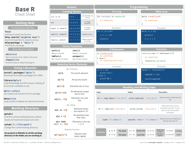
Reference Materials
Cheat Sheets
Further Reading
- R for Data Science, by Garrett Grolemund and Hadley Wickham.
- Advanced R, by Hadley Wickham.
Related DataCamp Courses
- Intermediate R (4 hours)
This content was presented to Nelson\Nygaard Staff at a Lunch and Learn webinar on Wednesday, February 17th, 2021, and is available as a recording here and embedded at the top of the page.