This content was presented to Nelson\Nygaard Staff at a Lunch and Learn webinar on Friday, October 2nd, 2020, and is available as a recording here and embedded below.

Soliciting Questions for the Final Course Module

Introduction

Acknowledgment: This module heavily draws upon, including direct copy-paste of markdown content, the vignettes developed for the tidytransit package, available on the package documentation website.

The General Transit Feed Specification

The summary page for the GTFS standard is a good resource for more information on the standard. GTFS was developed as a standardized way of publishing transit information for consumption by third-party applications (e.g., Google Maps). It is was originally developed as a collaboration between Google and TriMet, and became an open source definition for transit information around the world. What is still often referred to as GTFS is now more specifically referred to as GTFS static, because there are additional data feeds related to GTFS that transit agencies use, including GTFS-realtime, which provides realtime vehicle positioning and arrival estimates to third party applications (e.g., Google Maps, Transit).

GTFS provides a standard way to describe transit networks that is useful for NN’s analyses – because of GTFS’s standardization, many blocks of code can be re-used between projects for specific agencies. It is also always publicly available by its nature (i.e. it is published to a public web location for apps to consume), and so there is no need to request route/stop/schedule/etc. information from a client. You just need to figure out which version of the GTFS feed you want to use for your analysis.

GTFS feeds contain many linked tables about published transit schedules about service schedules, trips, stops, and routes. Below is a diagram of these relationships and tables:

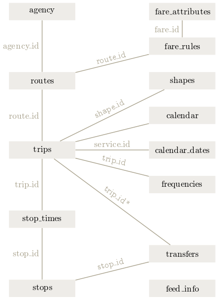gtfs-relationship-diagram Source: Wikimedia, user -stk.

Read a GTFS Feed

GTFS data come packaged as a zip file of tables in text form. The first thing tidytransit does is consolidate the reading of all those tables into a single R object, which contains a list of the tables in each feed. Below we use the tidytransit read_gtfs function in order to read a feed from TriMet into R.

I downloaded this feed to this course module’s data folder prior to running this code – you could also read the ZIP file directly from a public web url. This is useful because there are many sources for GTFS data, and often the best source is transit service providers themselves. See the next section on “Finding More GTFS Feeds” for more sources of feeds.

library(tidyverse)
library(sf)
library(tidytransit)
library(lubridate)
library(leaflet)

pdx <- read_gtfs("data/trimet_gtfs.zip")

You can use summary to get an overview of the feed.

summary(pdx)

GTFS object
files        agency, stops, routes, trips, stop_times, calendar, calendar_dates, fare_attributes, fare_rules, shapes, transfers, feed_info, route_directions, stop_features, linked_datasets
agencies     TriMet, Portland Streetcar, Port of Portland
service      from 2020-09-13 to 2020-12-05
uses         stop_times (no frequencies)
# routes        95
# trips      35813
# stop_ids    6791
# stop_names  4669
# shapes      1082

Each of the source tables for the GTFS feed is now available in the nyc gtfs object. For example, stops:

head(pdx$stops)

# A tibble: 6 x 13
  stop_id stop_code stop_name   stop_desc    stop_lat stop_lon zone_id
  <chr>   <chr>     <chr>       <chr>           <dbl>    <dbl> <chr>  
1 2       2         A Ave & Ch~ Eastbound s~     45.4    -123. B      
2 3       3         A Ave & Se~ Eastbound s~     45.4    -123. B      
3 4       4         A Ave & 10~ Westbound s~     45.4    -123. B      
4 6       6         A Ave & 8t~ Eastbound s~     45.4    -123. B      
5 7       7         A Ave & 8t~ Westbound s~     45.4    -123. B      
6 8       8         900 Block ~ Eastbound s~     45.4    -123. B      
# ... with 6 more variables: stop_url <chr>, location_type <int>,
#   parent_station <chr>, tts_stop_name <chr>, direction <chr>,
#   position <chr>

The tables available on each feed may vary. Below we can simply print the names of all the tables that were read in for this feed. Each of these is a table.

names(pdx)

 [1] "agency"           "calendar"         "calendar_dates"  
 [4] "fare_attributes"  "fare_rules"       "feed_info"       
 [7] "routes"           "route_directions" "shapes"          
[10] "stops"            "stop_features"    "stop_times"      
[13] "transfers"        "trips"            "linked_datasets" 
[16] "."

Finding GTFS Feeds

You can find current GTFS feeds through the tidytransit package directly as described on the documentation website. Nevertheless, I like to browse the feeds at transitfeeds.com, because this lets me easily browse for the specific vintage of feed that I am interested in. GTFS feeds are updated fairly often, especially for large agencies. This means that you may want to look at a previous version of the feed for your analysis, because schedules, routes, stops, or identifiers may have changed.

Understanding Service Periods

Overview

Each trip in a GTFS feed is referenced to a service_id (in trips.txt). The GTFS reference specifies that a “service_id contains an ID that uniquely identifies a set of dates when service is available for one or more routes”. A service could run on every weekday or only on Saturdays for example. Other possible services run only on holidays during a year, independent of weekdays. However, feeds are not required to indicate anything with service_ids and some feeds even use a unique service_id for each trip and day. In this vignette we’ll look at a general way to gather information on when trips run by using “service patterns”.

Service patterns can be used to find a typical day for further analysis like routing or trip frequencies for different days.

Prepare data

We’re going to again be using TriMet for our example.

gtfs <- read_gtfs("data/trimet_gtfs.zip")

Tidytransit provides a dates_services (stored in the list .) that indicates which service_id runs on which date. This is later useful for linking dates and trips via service_id.

head(gtfs$.$dates_services)

# A tibble: 6 x 2
  date       service_id
  <date>     <chr>     
1 2020-11-26 X.578     
2 2020-10-03 S.578     
3 2020-10-10 S.578     
4 2020-10-17 S.578     
5 2020-10-24 S.578     
6 2020-10-31 S.578

To understand service patterns better we need information on weekdays and holidays. With a calendar table we know the weekday and possible holidays for each date. We’ll use a minimal example with two holidays for Thanksgiving and Black Friday.

holidays = tribble(~date, ~holiday,
  ymd("2020-11-26"), "Thanksgiving",
  ymd("2020-11-27"), "Black Friday")
calendar = tibble(date = unique(gtfs$.$dates_services$date)) %>% 
  mutate(
    weekday = weekdays(date)
  )
calendar <- calendar %>% left_join(holidays, by = "date")
head(calendar)

# A tibble: 6 x 3
  date       weekday  holiday     
  <date>     <chr>    <chr>       
1 2020-11-26 Thursday Thanksgiving
2 2020-10-03 Saturday <NA>        
3 2020-10-10 Saturday <NA>        
4 2020-10-17 Saturday <NA>        
5 2020-10-24 Saturday <NA>        
6 2020-10-31 Saturday <NA>

To analyze on which dates trips run and to group similar services we use service patterns. Such a pattern simply lists all dates a trip runs on. For example, a trip with a pattern like 2019-03-07, 2019-03-14, 2019-03-21, 2019-03-28 runs every Thursday in March 2019. To handle these patterns we create a servicepattern_id using a hash function. Ideally there are the same number of servicepattern_ids and service_ids. However, in real life feeds, this is rarely the case. In addition, the usability of service patterns depends largely on the feed and its complexity.

gtfs <- set_servicepattern(gtfs)

Our gtfs feed now contains the data frame servicepatterns which links each servicepattern_id to an existing service_id (and by extension trip_id).

head(gtfs$.$servicepatterns)

# A tibble: 6 x 2
  service_id servicepattern_id
  <chr>      <chr>            
1 1.577      s_bbb6e9d        
2 1.578      s_911e55f        
3 2.577      s_5b651a0        
4 2.578      s_55fef4a        
5 3.577      s_6e70375        
6 3.578      s_05103f5

In addition, gtfs$.$dates_servicepatterns has been created which connects dates and service patterns (like dates_services). We can compare the number of service patterns to the number of services.

# service ids used
n_services <-  length(unique(gtfs$trips$service_id)) # 31
# unique date patterns 
n_servicepatterns <- length(unique(gtfs$.$servicepatterns$servicepattern_id)) # 16

The feed uses 31 service_ids but there are actually only 16 different date patterns. Other feeds might not have such low numbers, for example the Swiss GTFS feed uses around 15,600 service_ids which all identify unique date patterns.

Analyze Data

Exploration Plot

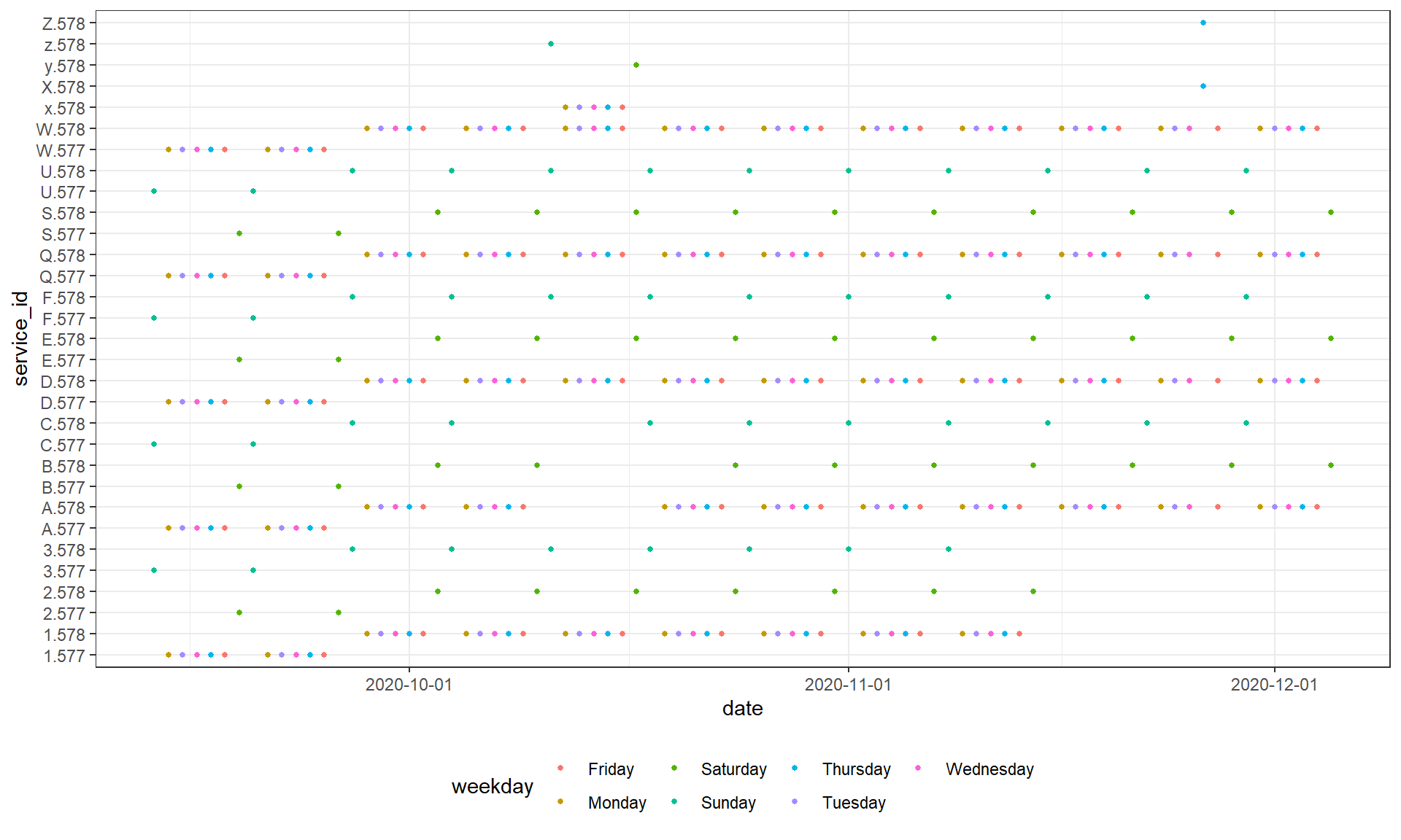
We’ll now try to figure out usable names for those patterns. A good way to start is visualizing the data.

date_servicepattern_table <- gtfs$.$dates_services %>% left_join(calendar, by = "date")
ggplot(date_servicepattern_table) + theme_bw() + 
  geom_point(aes(x = date, y = service_id, color = weekday), size = 1) + 
  scale_x_date(breaks = scales::date_breaks("1 month")) + theme(legend.position = "bottom")

Names for service patterns

It’s generally difficult to automatically generate readable names for service patterns. Below you see a semi automated approach with some heuristics. However, the workflow depends largely on the feed and its structure. You might also consider setting names completely manually.

suggest_servicepattern_name = function(dates, calendar) {
  servicepattern_calendar = tibble(date = dates) %>% left_join(calendar, by = "date")
  
  # all normal dates without holidays
  calendar_normal = servicepattern_calendar %>% filter(is.na(holiday))
  
  # create a frequency table for all calendar dates without holidays
  weekday_freq = sort(table(calendar_normal$weekday), decreasing = T)
  n_weekdays = length(weekday_freq)
  
  # all holidays that are not covered by normal weekdays anyways
  calendar_holidays <- servicepattern_calendar %>% filter(!is.na(holiday)) %>% filter(!(weekday %in% names(weekday_freq)))
  if(n_weekdays == 7) {
    pattern_name = "Every day"
  }
  # Single day service
  else if(n_weekdays == 1) {
    wd = names(weekday_freq)[1]
    # while paste0(weekday, "s") is easier, this solution can be used for other languages
    pattern_name = c("Sunday"  = "Sundays", 
        "Monday"    = "Mondays", 
        "Tuesday"   = "Tuesdays", 
        "Wednesday" = "Wednesdays",
        "Thursday"  = "Thursdays",  
        "Friday"    = "Fridays",  
        "Saturday"  = "Saturdays")[wd]
  } 
  # Weekday Service
  else if(n_weekdays == 5 && 
      length(intersect(names(weekday_freq), 
        c("Monday", "Tuesday", "Wednesday", "Thursday", "Friday"))) == 5) {
    pattern_name = "Weekdays"
  }
  # Weekend
  else if(n_weekdays == 2 && 
      length(intersect(names(weekday_freq), c("Saturday", "Sunday"))) == 2) {
    pattern_name = "Weekends"
  }
  # Multiple weekdays that appear regularly
  else if(n_weekdays >= 2 && (max(weekday_freq) - min(weekday_freq)) <= 1) {
    wd = names(weekday_freq)
    ordered_wd = wd[order(match(wd, c("Monday", "Tuesday", "Wednesday", "Thursday", "Friday", "Saturday", "Sunday")))]
    pattern_name = paste(ordered_wd, collapse = ", ")
  } 
  # default
  else {
    pattern_name = paste(weekday_freq, names(weekday_freq), sep = "x ", collapse = ", ")
  }
  
  # add holidays
  if(nrow(calendar_holidays) > 0) {
    pattern_name <- paste0(pattern_name, " and ", paste(calendar_holidays$holiday, collapse = ", "))
  }
  
  pattern_name <- paste0(pattern_name, " (", min(dates), " - ", max(dates), ")") 
  return(pattern_name)
}

We’ll apply this function to our service patterns and create a table with ids and names.

servicepattern_names = gtfs$.$dates_services %>% 
  group_by(service_id) %>% summarise(
    servicepattern_name = suggest_servicepattern_name(date, calendar)
  )
print(servicepattern_names)

# A tibble: 31 x 2
   service_id servicepattern_name                
   <chr>      <chr>                              
 1 1.577      Weekdays (2020-09-14 - 2020-09-25) 
 2 1.578      Weekdays (2020-09-28 - 2020-11-13) 
 3 2.577      Saturdays (2020-09-19 - 2020-09-26)
 4 2.578      Saturdays (2020-10-03 - 2020-11-14)
 5 3.577      Sundays (2020-09-13 - 2020-09-20)  
 6 3.578      Sundays (2020-09-27 - 2020-11-08)  
 7 A.577      Weekdays (2020-09-14 - 2020-09-25) 
 8 A.578      Weekdays (2020-09-28 - 2020-12-04) 
 9 B.577      Saturdays (2020-09-19 - 2020-09-26)
10 B.578      Saturdays (2020-10-03 - 2020-12-05)
# ... with 21 more rows

Visualize services

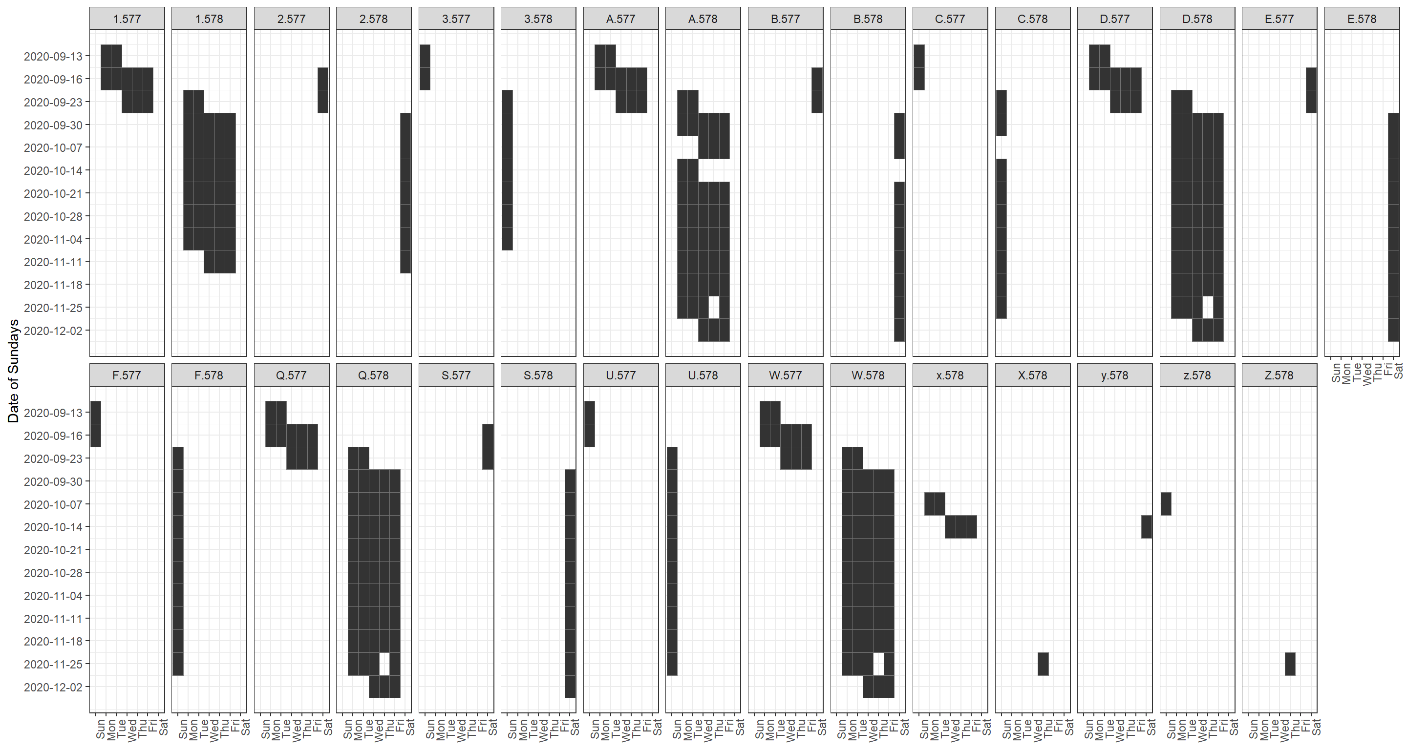
Plot calendar for each service pattern

We can plot the service pattern like a calendar to visualise the different patterns. The original services can be plotted similarly (given it’s not too many) by using date_service_table and service_id.

dates = gtfs$.$dates_services
dates$wday <- lubridate::wday(dates$date, label = T, abbr = T, week_start = 7)
dates$week_nr <- lubridate::week(dates$date)
dates <- dates %>% group_by(week_nr) %>% summarise(week_first_date = min(date)) %>% right_join(dates, by = "week_nr")
week_labels = dates %>% select(week_nr, week_first_date) %>% unique()
ggplot(dates) + theme_bw() +
  geom_tile(aes(x = wday, y = week_nr), color = "#747474") +
  scale_x_discrete(drop = F) +
  scale_y_continuous(trans = "reverse", labels = week_labels$week_first_date, breaks = week_labels$week_nr) +
  theme(legend.position = "bottom", axis.text.x = element_text(angle = 90, hjust = 1)) +
  labs(x = NULL, y = "Date of Sundays") +
  facet_wrap(~service_id, nrow = 2)

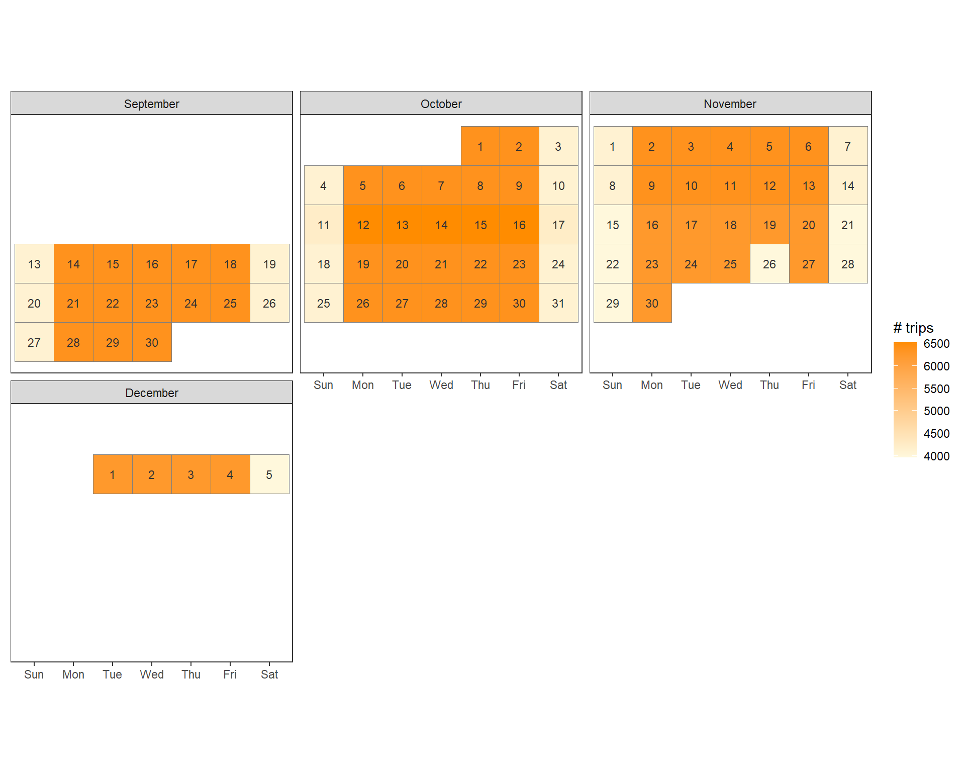
Plot number of trips per day as calendar

We can plot the number of trips for each day as a calendar heat map.

trips_servicepattern = left_join(select(gtfs$trips, trip_id, service_id), gtfs$.$servicepatterns, by = "service_id")
trip_dates = left_join(gtfs$.$dates_services, trips_servicepattern, by = "service_id")
trip_dates_count = trip_dates %>% group_by(date) %>% summarise(count = dplyr::n()) 
trip_dates_count$weekday <- lubridate::wday(trip_dates_count$date, label = T, abbr = T, week_start = 7)
trip_dates_count$day_of_month <- lubridate::day(trip_dates_count$date)
trip_dates_count$first_day_of_month <- lubridate::wday(trip_dates_count$date - trip_dates_count$day_of_month,  week_start = 7)
trip_dates_count$week_of_month <- ceiling((trip_dates_count$day_of_month - as.numeric(trip_dates_count$weekday) - trip_dates_count$first_day_of_month) / 7)
trip_dates_count$month <- lubridate::month(trip_dates_count$date, label = T, abbr = F)
ggplot(trip_dates_count, aes(x = weekday, y = -week_of_month)) + theme_bw() +
  geom_tile(aes(fill = count, colour = "grey50")) +
  geom_text(aes(label = day_of_month), size = 3, colour = "grey20") +
  facet_wrap(~month, ncol = 3) +
  scale_fill_gradient(low = "cornsilk1", high = "DarkOrange", na.value="white")+
    scale_color_manual(guide = F, values = "grey50") +
  theme(axis.text.y = element_blank(), axis.ticks.y = element_blank()) +
  theme(panel.grid = element_blank()) +
  labs(x = NULL, y = NULL, fill = "# trips") +
  coord_fixed()

Headway Mapping

Import Transit Data (GTFS)

We’ll again start by importing a snapshot of TriMet’s GTFS.

gtfs <- read_gtfs("data/trimet_gtfs.zip")

Identify Weekday Schedules of Service

GTFS feeds typically contain a schedule of all the schedules of service for a given system. Selecting a schedule of service in Portland allows us to focus on, for example, non-holiday weekday service, in the Fall of 2020. In some feeds, service selection can be more or less complicated than Portland. In any case, the work we did above in identifying service patterns is helpful.

gtfs <- set_servicepattern(gtfs)

After setting the service patterns, we can summarise each service by the number of trips and stops. We’ll also summarise the total distance covered by all trips in the service, and then check that against the total distance covered by the average route. First, we need to calculate the distance of each part of the route shapes.

shp1 <- shapes_as_sf(gtfs$shapes)
shp1 <- st_transform(shp1, crs=2269)
shp1$length <- st_length(shp1)
shp2 <- shp1 %>% 
  as.data.frame() %>% 
  select(shape_id,length,-geometry)

Now we’re ready to roll the statistics up to services.

service_pattern_summary <- gtfs$trips %>%
  left_join(gtfs$.$servicepatterns, by="service_id") %>% 
  left_join(shp2, by="shape_id") %>%
  left_join(gtfs$stop_times, by="trip_id") %>% 
  group_by(service_id) %>% 
  summarise(trips = n(), 
            routes = n_distinct(route_id),
            total_distance_per_day_mile = sum(as.numeric(length), 
                                    na.rm=TRUE)/5280,
            route_avg_distance_mile = (sum(as.numeric(length),
                                    na.rm=TRUE)/5280)/(trips*routes),
            stops=(n_distinct(stop_id)/2))

We can also add the number of days that each service is in operation, and the service pattern names we established above.

service_pattern_summary <- gtfs$.$dates_services %>% 
  group_by(service_id) %>% 
  summarise(days_in_service = n()) %>% 
  left_join(service_pattern_summary, by="service_id") %>%
  left_join(servicepattern_names)

And then we’ll print the summary.

knitr::kable(service_pattern_summary)

service_id	days_in_service	trips	routes	total_distance_per_day_mile	route_avg_distance_mile	stops	servicepattern_name
1.577	10	286	1	696.1951	2.4342485	1.0	Weekdays (2020-09-14 - 2020-09-25)
1.578	35	286	1	696.1951	2.4342485	1.0	Weekdays (2020-09-28 - 2020-11-13)
2.577	2	284	1	690.8280	2.4324930	1.0	Saturdays (2020-09-19 - 2020-09-26)
2.578	7	284	1	690.8280	2.4324930	1.0	Saturdays (2020-10-03 - 2020-11-14)
3.577	2	266	1	647.5452	2.4343805	1.0	Sundays (2020-09-13 - 2020-09-20)
3.578	7	266	1	647.5452	2.4343805	1.0	Sundays (2020-09-27 - 2020-11-08)
A.577	10	17217	5	341812.5606	3.9706402	80.5	Weekdays (2020-09-14 - 2020-09-25)
A.578	44	17217	5	341812.5606	3.9706402	80.5	Weekdays (2020-09-28 - 2020-12-04)
B.577	2	15398	5	300225.7579	3.8995423	80.5	Saturdays (2020-09-19 - 2020-09-26)
B.578	9	15398	5	300225.7579	3.8995423	80.5	Saturdays (2020-10-03 - 2020-12-05)
C.577	2	15398	5	300225.7579	3.8995423	80.5	Sundays (2020-09-13 - 2020-09-20)
C.578	9	15398	5	300225.7579	3.8995423	80.5	Sundays (2020-09-27 - 2020-11-29)
D.577	10	5179	3	26922.3747	1.7327911	36.0	Weekdays (2020-09-14 - 2020-09-25)
D.578	49	5179	3	26922.3747	1.7327911	36.0	Weekdays (2020-09-28 - 2020-12-04)
E.577	2	4685	3	24217.2072	1.7230315	36.0	Saturdays (2020-09-19 - 2020-09-26)
E.578	10	4685	3	24217.2072	1.7230315	36.0	Saturdays (2020-10-03 - 2020-12-05)
F.577	2	4685	3	24217.2072	1.7230315	36.0	Sundays (2020-09-13 - 2020-09-20)
F.578	10	4685	3	24217.2072	1.7230315	36.0	Sundays (2020-09-27 - 2020-11-29)
Q.577	10	100	1	1456.1977	14.5619769	3.0	Weekdays (2020-09-14 - 2020-09-25)
Q.578	49	100	1	1456.1977	14.5619769	3.0	Weekdays (2020-09-28 - 2020-12-04)
S.577	2	202825	47	3012243.6372	0.3159881	2411.0	Saturdays (2020-09-19 - 2020-09-26)
S.578	10	202808	47	3014533.7727	0.3162549	2410.5	Saturdays (2020-10-03 - 2020-12-05)
U.577	2	202825	47	3012243.6372	0.3159881	2411.0	Sundays (2020-09-13 - 2020-09-20)
U.578	10	202808	47	3014533.7727	0.3162549	2410.5	Sundays (2020-09-27 - 2020-11-29)
W.577	10	319583	84	4588160.2460	0.1709132	3246.5	Weekdays (2020-09-14 - 2020-09-25)
W.578	49	319563	84	4590990.3024	0.1710293	3246.0	Weekdays (2020-09-28 - 2020-12-04)
x.578	5	17397	6	305117.1921	2.9230824	81.5	Weekdays (2020-10-12 - 2020-10-16)
X.578	1	202808	47	3014533.7727	0.3162549	2410.5	and Thanksgiving (2020-11-26 - 2020-11-26)
y.578	1	15538	6	268569.3856	2.8807803	81.5	Saturdays (2020-10-17 - 2020-10-17)
z.578	1	15538	6	268569.3856	2.8807803	81.5	Sundays (2020-10-11 - 2020-10-11)
Z.578	1	20215	8	330982.5637	2.0466396	117.0	and Thanksgiving (2020-11-26 - 2020-11-26)

It seems that if we want to summarise the most common patterns of service in the TriMet system, we should use the W.577 service ID, as it has the most days in service, the most trips, stops, and routes.

Calculate Headways

So, now that we’ve used service patterns to identify the set of service_id’s that refer to all weekday trips, we can summarize service between 6 am and 10 am for the TriMet System on weekdays.

am_freq <- get_stop_frequency(gtfs, start_hour = 6, end_hour = 10, service_ids = c("W.577"), by_route = TRUE)

knitr::kable(head(am_freq))

stop_id	route_id	direction_id	service_id	n_departures	mean_headway
10	34	0	W.577	3	4800
100	88	1	W.577	8	1800
10000	46	1	W.577	4	3600
10001	46	1	W.577	3	4800
10004	46	0	W.577	3	4800
10005	46	0	W.577	3	4800

This table includes columns for the id for a given stop, the route_id (because we used the by_route parameter), our selected service_id’s, and the number of departures and the average headway for a given direction from 6 am to 10 am on weekdays.

The get_stop_frequency function simply counts the number of departures within the time frame to get departures per stop. Then, to get headways, it divides the number of minutes by the number of departures, and rounds to the nearest integer.

Lets have a look at the headways for route 4, which runs from downtown Portland to Saint Johns, a neighborhood at the far edge of North Portland.

First, we filter the am_freq data frame to just stops going in 1 direction on the 1 bus, and then we join to the original stops table, which includes a more descriptive stop_name.

one_line_stops <- am_freq %>% 
    filter(route_id==4 & direction_id==0) %>%
    left_join(gtfs$stops, by ="stop_id")

Lets also plot the headways at these stops on a map to see how they are distributed across the city. First, we’ll use the stops_as_sf function, which converts the latitudes and longitudes on the stops table in the GTFS feed into simple features.

pdx_stops_sf <- stops_as_sf(gtfs$stops)

Now we can join those stop coordinates to the calculated stop headways.

one_line_stops_sf <- pdx_stops_sf %>%
  right_join(one_line_stops, by="stop_id")

And then use ggplot’s geom_sf to plot the headways.

one_line_stops_sf %>% 
  ggplot() + 
  geom_sf(aes(color=mean_headway)) +
  theme_bw()

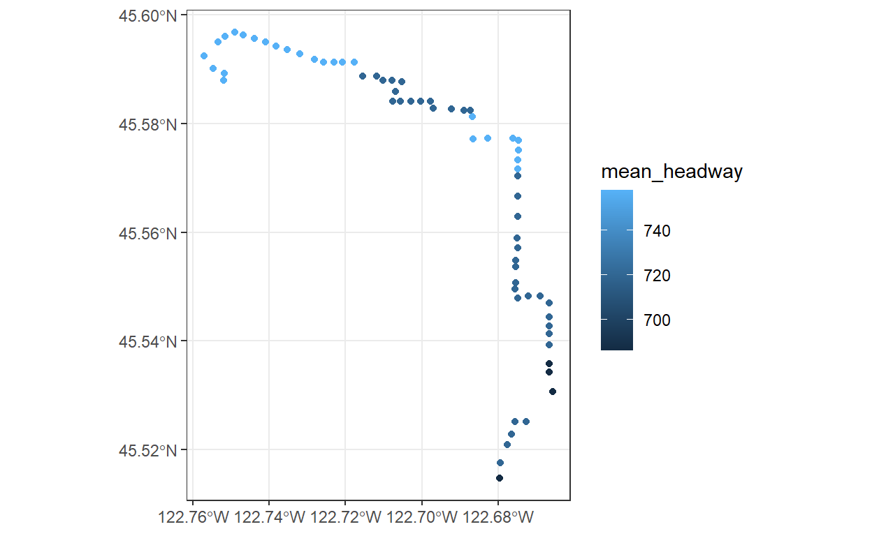
Finally, we can easily summarise what the headways are like along the entire route now, by using r’s default summary function for the vector of headways.

summary(one_line_stops$mean_headway)

   Min. 1st Qu.  Median    Mean 3rd Qu.    Max. 
  686.0   720.0   720.0   732.7   758.0   758.0

Headways over Time

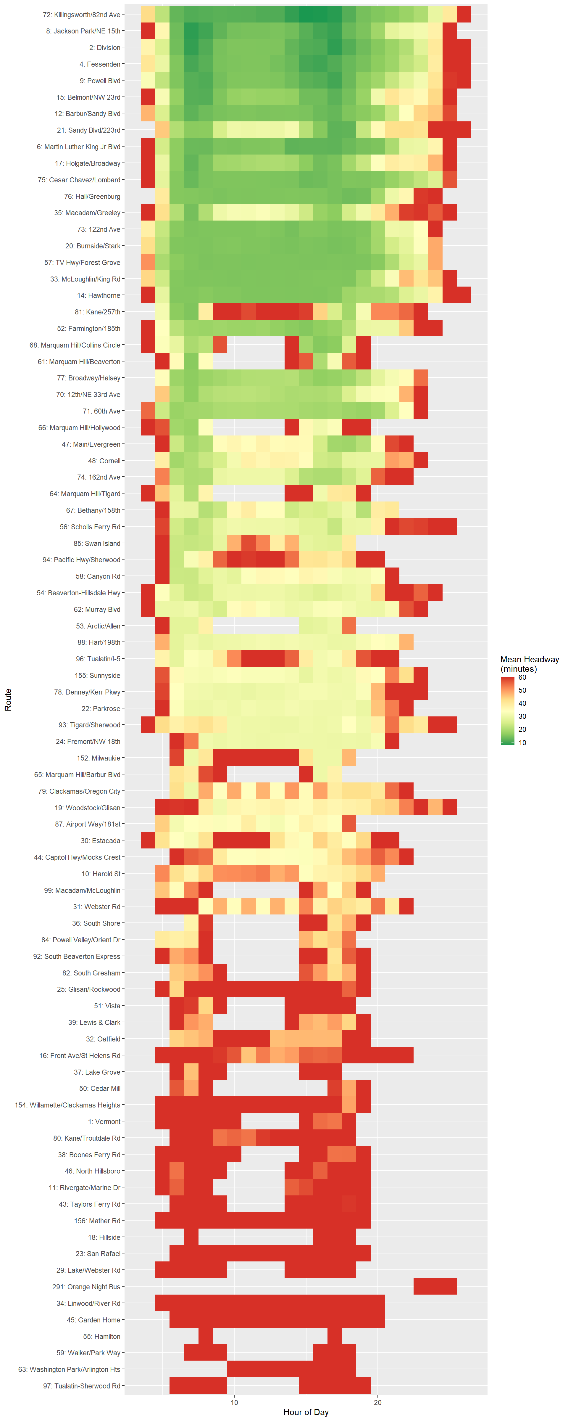
We can also plot frequency at different times of day. To keep it simpler, we will do this for just one service pattern, as above.

#Filter only for trips in those service IDs
sub_trips = gtfs$trips %>%
  filter(service_id == 'W.577') 

#Join in trip and route metadata (including route names)
sub_stop_times = gtfs$stop_times %>%
  filter(trip_id %in% sub_trips$trip_id) %>%
  left_join(sub_trips) %>%
  left_join(gtfs$routes) %>%
  mutate(depart_hour = str_sub(departure_time,1,2) %>%
           as.numeric())

#Calculate mean headway within each route, averaging across stop and direction
summ_freq = sub_stop_times %>%
  group_by(route_id,route_short_name,route_long_name,direction_id,depart_hour,stop_id) %>%
  summarise(num_departs = n()) %>%
  ungroup() %>%
  group_by(route_id,route_short_name,route_long_name,depart_hour) %>%
  summarise(avg_departs = mean(num_departs)) %>%
  mutate(avg_headway = 60/avg_departs) %>%
  ungroup() %>%
  mutate(route_label = paste0(route_short_name,': ',route_long_name)) %>%
  arrange(desc(avg_departs)) %>%
  mutate(route_label = factor(route_label,ordered=TRUE,levels = rev(unique(route_label))))

#Plot using the geom_tile function, which plots identically sized rectangles that can be filled based on an aesthetic
ggplot(summ_freq,aes(x=depart_hour,y = route_label,fill=avg_headway))+
  geom_tile()+
  scale_fill_distiller(palette = 'RdYlGn',name='Mean Headway\n(minutes)')+
  xlab('Hour of Day')+
  ylab('Route')

Wrap Up

There is a lot you can do with GTFS data – our transit dashboards we have built for TriMet and are building for other agencies heavily rely on the standardization of GTFS. They provide great datasets to test the R skills you are learning on for something very relevant to our work! Remix outputs scenarios developed in the tool directly in GTFS. Drafting up new transit services in a GTFS-like format can help you to compare existing service with new service. There are a lot of ideas to explore in your work with GTFS, and R makes handling the multiple tables and the spatial/aspatial nature of GTFS easier.

This content was presented to Nelson\Nygaard Staff at a Lunch and Learn webinar on Friday, October 2nd, 2020, and is available as a recording here and embedded at the top of the page.

GTFS Data