This content was presented to Nelson\Nygaard Staff at a GIS Hangout on Thursday, January 21st, 2021, and is available as a recording here and embedded below.
Background
For those that have been using R at NN for several years, you may be familiar with querying travel times using functions in the transportr package – a bare bones package Bryan was saving useful functions into for NN R work. Back in 2016, when Bryan was writing a function for querying Google Directions, there was no existing package/function for doing so. In the intervening years, other packages have been developed that are more fully featured and better maintained than the corresponding functions in transportr.
Going forward, it is recommended that you use the googleway package, which provides a variety of functions for interacting with various Google Maps APIs, including querying travel times. This tutorial will demonstrate the usage of this package for querying auto travel times and then adjusting them based on travel pattern changes due to the COVID-19 pandemic. Future trainings will discuss the use of this package for querying travel times for other modes, and likely other Google APIs as well.
This tutorial draws upon code snippets from the googleway vignette – if you want a full guide to all the features of the package, please refer to that. We will focus on a couple of examples for travel time querying below.
Basic Usage
Setting up an API Key
The first thing you need to do to work with Google’s APIs (Application Programming Interface) is create your own API key so that your API calls can be tracked. Google does this because this is a service that they charge for if you do more than a couple thousand calls per day (each API has its own usage tiers). You can create your own key by going to the Google Developer Console, logging in with an account (I use an account linked to my NN email address), and then creating an initial API key in the ‘Credentials’ panel. It is helpful if you have multiple projects using APIs to create a key per project, as this will be easier to separate for billing purposes. You will need to provide a credit card for Google to charge to in order to use APIs – they will only charge your credit card if you go beyond the free usage tier, in which case you should be expensing those charges to a project. For practice, we shouldn’t need to go over the free usage tier.
After creating a key, you must enable API services tied to that key. For this tutorial, it is recommended you enable the following API services:
- Directions API – the main API we are using to query directions (and the travel times attached to them)
- Maps Javascript API – the API used to generate the interactive Google map widgets used in this tutorial for visualization purposes
- Geocoding API – this is activated so that you can insert addressed into the
google_directions()function. Addresses and place names need to be geocoded prior to evaluation.
After you enable the APIs, use the below line of code to set your API key to be used by the googleway package. Prior, we must load the packages we will be using in this tutorial.
#Using an API Key set up for NN R training -- please use your own API key oelow
set_key('<YOUR API KEY HERE>')
Example Trip Queries
Below we will demonstrate the usage of the Directions API for querying directions/travel times for an AM and PM commute from a randomly selected suburban location in Vancouver, WA to the SmartPark parking garage near Nelson\Nygaard’s office in Downtown Portland (OR). You will notice that the queried date for directions is June 1, 2021 – the query date/time must always be in the future. If you do not select a date/time, the function will default to the current time when the function is called. There is no way to query directions in the past. This date was chosen to represent an arbitrarily chosen Tuesday at some point in the future. Google’s estimates are based on historical data, but we do not know how the past months of the COVID-19 pandemic have affected that historical data being drawn upon – local judgment will have to be used when evaluating and/or adjusting these travel times.
AM Commute
The AM commmute is assumed to depart at 7:30 am – obviously assuming for the sake of example that people are back to commuting regularly. We set the origin and destination by manually inserting the latitude/longitude coordinates of the locations – you could use an address as well, but this would need to be geocoded (which would be done behind the scenes in the function). You also select the mode (driving), hand the function a departure timestamp (coerced into POSIXct, a time format), and then specify that we want to see multiple alternatives if they exist, not just the optimal route selected.
We print the results of the function to show you what they look like – a list containing a lot of information including the shape of the route, the travel time, text descriptions of the steps for the route, etc. All this information is provided because people use this API for many purposes, including third-party apps that rely on the directions API to provide travel directions. You will notice that the polyline shape is returned as an encoded text string – this is a method of compressing the data for transfer over the web. You can use the decode_pl() function to decode the text string into a series of lat/lon vertices describing the polyline. We use several map() functions throughout this tutorial – if these are unfamiliar to you, please refer to the other tutorials on the subject provided on this site.
Google directions (for the driving mode) will return a duration and a duration_in_traffic – you can interpret the duration as the free flow travel time, and the duration_in_traffic as the estimated travel time based on the predicted amount of congestion on the roadway at the query time. As we will use later on in the tutorial, we can calculate the ratio of the duration_in_traffic to duration as the travel time index – a ratio between travel time in the congested peak and the free flow travel time. The AM commute here is predicted to be relatively uncongested given the low travel time indices (between 1 and 1.1) – this is almost certainly a COVID-19 pandemic-related effect.
In the final line of code below, we use the google_map() function to create an interative Google Map widget, on which we can plot the polylines representing our routes.
dir_results_am = google_directions(origin = '45.63039565205174, -122.58032084515692',
                  destination = '45.51969205229432, -122.6822162060739',
                  mode = 'driving',
                  departure_time = as.POSIXct('2021-06-01 07:30:00', tz='America/Los_Angeles'),
                  alternatives = TRUE)

print(dir_results_am)
$geocoded_waypoints
geocoder_status place_id types
1 OK ChIJQ51tM3ellVQRQUSUWhU8cvA premise
2 OK ChIJ85UqugQKlVQRD4O-PmY6nf4 street_address
$routes
bounds.northeast.lat bounds.northeast.lng bounds.southwest.lat
1 45.63147 -122.5795 45.51934
2 45.63110 -122.5438 45.51746
bounds.southwest.lng copyrights
1 -122.6875 Map data ©2021
2 -122.6828 Map data ©2021
legs
1 22.7 km, 22709, 23 mins, 1370, 24 mins, 1442, 740 SW 10th Ave, Portland, OR 97205, USA, 45.5197152, -122.6822678, 1205 NE Cedar Ridge Loop, Vancouver, WA 98664, USA, 45.6302853, -122.5803194, 62 m, 77 m, 80 m, 0.1 km, 0.2 km, 0.2 km, 0.7 km, 0.2 km, 1.3 km, 6.5 km, 9.4 km, 1.0 km, 0.8 km, 1.0 km, 0.3 km, 51 m, 0.3 km, 0.4 km, 45 m, 62, 77, 80, 132, 235, 162, 665, 153, 1288, 6485, 9440, 989, 810, 989, 339, 51, 286, 421, 45, 1 min, 1 min, 1 min, 1 min, 1 min, 1 min, 1 min, 1 min, 2 mins, 4 mins, 6 mins, 1 min, 1 min, 1 min, 1 min, 1 min, 1 min, 2 mins, 1 min, 8, 27, 22, 27, 39, 27, 77, 19, 137, 240, 388, 41, 34, 42, 34, 13, 72, 104, 19, 45.6302902, 45.6307447, 45.631468, 45.6311204, 45.6290707, 45.6290489, 45.6230679, 45.623287, 45.6117051, 45.6208255, 45.5487194, 45.5408636, 45.5353545, 45.5265836, 45.5235657, 45.5231178, 45.5206867, 45.5193372, 45.5197152, -122.5795233, -122.5800627, -122.5800541, -122.581628, -122.5815971, -122.5836823, -122.5836032, -122.5855509, -122.5856419, -122.6668709, -122.6787789, -122.6795613, -122.6863679, -122.6869077, -122.6867258, -122.6866048, -122.6875299, -122.6824859, -122.6822678, Head <b>east</b> on <b>NE 12th Dr</b> toward <b>NE Cedar Ridge Loop</b>, Turn <b>left</b> onto <b>NE Cedar Ridge Loop</b>, Turn <b>right</b> to stay on <b>NE Cedar Ridge Loop</b>, Turn <b>left</b> onto <b>NE 13th St</b>, Continue onto <b>NE 89th Ave</b>, Turn <b>right</b> onto <b>NE 11th St</b>, Turn <b>left</b> onto <b>NE 87th Ave</b>, Turn <b>right</b> onto <b>E Mill Plain Blvd</b>, Turn <b>left</b> onto <b>N Lieser Rd</b>, Turn <b>right</b> to merge onto <b>WA-14 W</b> toward <b>I-5</b>/<wbr/><b>City Center</b>, Take the exit on the <b>left</b> onto <b>I-5 S</b> toward <b>Portland</b><div style="font-size:0.9em">Entering Oregon</div>, Take exit <b>302B</b> for <b>I-405</b>/<wbr/><b>US-30 W</b> toward <b>Beaverton</b>/<wbr/><b>St. Helens</b>, Continue onto <b>I-405 S</b>/<wbr/><b>US-30 W</b>, Keep <b>left</b> to continue on <b>I-405 S</b>, follow signs for <b>US-26 W</b>/<wbr/><b>City Center</b>/<wbr/><b>Beaverton</b>/<wbr/><b>Glisan St</b>/<wbr/><b>Everett St</b>, Take exit <b>2 A</b> for <b>Couch St</b> toward <b>Burnside St</b>, Continue onto <b>NW 15th Ave</b>, Continue straight onto <b>S 15th Ave</b>, Turn <b>left</b> onto <b>S Yamhill St</b>, Turn <b>left</b> onto <b>SW 10th Ave</b><div style="font-size:0.9em">Destination will be on the right</div>, idouG~mdkV?w@?s@?s@, idouG~hdkVe@@C?C@C@CBCBC@A@ABCBCBABABABAD?FAFAJALAP, cgouGjldkVc@?c@@e@Ac@A, ukouGhldkV@nBBRDVBX@HJ^Nj@Vn@, oiouGdvdkVVPLJRJ\\FB?V@P?P?b@?T?JAL?NCLCHEJEHCDC@AHCFCHEJCHAFANALAN?, u|nuG~udkV@xC@dG, q|nuG~bekVlB@d@ApBGfA?D?|ABVAV?b@?`@?tEAl@Ab@Cb@@PAt@?L?P?hAAT?nB?, ewmuGnbekVIdBC`@OfCMtB, qxmuGtnekVv@?`@?jA@tB@jFBt@?`A?T?d@?J?`FDvA?rB?b@?b@An@?X?Z?b@?VBrACVAd@AdA?dA?bA@fA?b@?pB?J?ZAX@r@Cz@DhABn@?~@@, epkuGfoekV?h@@t@?r@Ap@?p@?v@Ab@?JANAV?JAPC\\I|@QdB?BAB?D@B@BDH_@jCGd@Ip@Ih@QbBMvAI|@Eb@Gx@Ch@Gz@Ev@KdCAL]tIg@pMKhCIzBIzAIvAGp@Gt@K|@Mz@U`BeBzKc@nCm@~D}@pFO`AETOjAM`ASrBQ~CGzAAx@Al@Ar@?dEA`AAx@Ct@OpCGv@A@K~@O|@SpA}CxNo@zCWfAMZa@rBw@~DSdASjACHKn@Ib@_@jCUdBQzACTW`CIdAGr@UtCOlBMbCABItBEtAEbBEdB?LA`BAxA?lDB|DD`G?tN?fBAnMAzS?d@@hEBrGNdR@xA?fD@dB@rE@rC@lE?pC?`@?L?T?z@?tA@`G@lBAtAAbCA\\?RCrAAh@ErAAZCp@GlAE`AGdAItAC\\KjAARCXq@vG]vCKx@It@Gl@Il@CVKz@Kx@O~@ObAMr@UhAS|@WhASv@CFMf@Wz@Ob@Sl@O`@Uj@, eimuG|jukVOb@M\\c@bA_@z@cArBm@hAw@|AWd@Ub@?@A@Ud@KXGLMTWh@Q`@CFS`@Sf@Sh@EJABABM\\CDELCB?@Sh@GNGNKVMPGJEFEFGFKHOFKBI@I?MAIAICMIIGGIIKGMEIEMCKCKAMAM?MAm@DUBKDIBIDGHMDGFEFGNILCF?FAJ?D?D@HBFBDBDBDBDFNPfAxALNT\\\\b@@@@@D@RJb@n@f@p@JJDFNPTTPPTNVTRHPJNH?@@?DBLH@?@@B@DB@@JF~@f@fEtB`Af@?@jIdEbBz@^P`@R^R`@R`Af@l@XTJbCnA`Af@`@PvAt@h@Vf@Vb@TVLNHHDZNRJRJZLJFD@ZNFBD@ZN\\LrB`AZLLF`Bp@xAl@`Br@b@T^RhAj@fAl@vAp@^T@?HDTLPFpBbApBbAbDpA@?fCx@B?PFLDj@Jj@JjCh@b@Jb@HLBVFB??@VD@?b@JXDzDv@h@JfAVh@JtAX\\JjF`AxEz@zAX`@DTDz@HtAFz@BX?P?N?T?dBEr@Kj@IdASf@K`A[LCf@OXKtCeAzJiDfDmAVI|@]|@Wz@[nBq@jAc@r@UdCy@hBm@d@S@?h@Ux@YjDoAlC_AfC}@vAg@XKLC\\KjAY|A[nAQtCWLAR?R?b@Ab@?b@?jB?`B?vC@J?p@Ar@?rC@lC?\\@hCBfAA|@@h@?dD@~B?`F@f@?tC?hF?rDCR?B?lDAb@?lBAv@?jA@tC@~AA@?rA@lC@xA?D?JAB?|FAx@A|AAtCCfQEhEBlC@hA?F?nA@`A?D@H?@?`ABJ?x@@L?J?lB?zCEzA?hC@fDBfC@nC@b@@bD@~C@, of_uGjuwkVNNB?BBB?f@?T?`A@J?B?X?LAV?F?ZCHA@?VETE^KXKDARIBANIPIBC@ALGNKDEROROJIBCXUXUDCBCVS@ADCLKj@c@b@_@FEBENKVQBAVQPKHEBAXK\\KLAHCTCB?P?VAP@J@VF`@LB?PHHFHD@@DDLHHHDBDBLLBDJLFFDD@Bh@r@JNBBV\\v@`Ad@j@PRX\\NPJN@@V\\?@Z\\LLRXPZ, ku}tGfzwkVBFHL@@HJDF@BjHnJnAdBpAbBr@~@x@dAlBbClBbCnBbCJP@@?@nAzAb@p@`@p@, }r|tGxdykVTDRJVXXVLHRLPJTJZJRDXHLBRDN@TBd@@H?@?tACzAA`@?bAC@?@?b@Ab@AB?^?\\A@?B?H?X?N@b@?p@@Z?^@^?jBEF?ZAxAChAEnAE`BCrAEVCn@?FAH?hAC, c|ztGdhykVJDF@VBZ?d@DdAFn@Bp@@z@A~@IxASdASf@O, iiztG`gykVb@IDA@?BAHA^I, ofztGffykVn@Md@EN?@?B@@?DBbAb@`@P\\N`Ab@`@RDB`A`@TJd@RDB, iwytG`lykVLs@X_BLo@N{@Nu@?CLo@Hk@X_BXeBJm@Hc@ZqB@Kj@uCJm@, {nytGplxkVGEcAe@, 45.6302853, 45.6302902, 45.6307447, 45.631468, 45.6311204, 45.6290707, 45.6290489, 45.6230679, 45.623287, 45.6117051, 45.6208255, 45.5487194, 45.5408636, 45.5353545, 45.5265836, 45.5235657, 45.5231178, 45.5206867, 45.5193372, -122.5803194, -122.5795233, -122.5800627, -122.5800541, -122.581628, -122.5815971, -122.5836823, -122.5836032, -122.5855509, -122.5856419, -122.6668709, -122.6787789, -122.6795613, -122.6863679, -122.6869077, -122.6867258, -122.6866048, -122.6875299, -122.6824859, DRIVING, DRIVING, DRIVING, DRIVING, DRIVING, DRIVING, DRIVING, DRIVING, DRIVING, DRIVING, DRIVING, DRIVING, DRIVING, DRIVING, DRIVING, DRIVING, DRIVING, DRIVING, DRIVING, NA, turn-left, turn-right, turn-left, NA, turn-right, turn-left, turn-right, turn-left, ramp-right, ramp-left, ramp-right, NA, keep-left, ramp-right, NA, straight, turn-left, turn-left
2 24.9 km, 24852, 24 mins, 1454, 26 mins, 1586, 740 SW 10th Ave, Portland, OR 97205, USA, 45.5197152, -122.6822678, 1205 NE Cedar Ridge Loop, Vancouver, WA 98664, USA, 45.6302853, -122.5803194, 80 m, 0.4 km, 0.9 km, 1.1 km, 10.9 km, 8.7 km, 0.6 km, 0.6 km, 0.5 km, 0.5 km, 0.3 km, 0.2 km, 0.1 km, 80, 367, 873, 1135, 10921, 8714, 564, 640, 458, 451, 318, 203, 128, 1 min, 1 min, 2 mins, 2 mins, 7 mins, 6 mins, 1 min, 1 min, 1 min, 2 mins, 1 min, 1 min, 1 min, 17, 80, 118, 125, 415, 342, 27, 36, 34, 92, 73, 54, 41, 45.63031, 45.6300293, 45.6221817, 45.6209459, 45.5352424, 45.5253795, 45.5222374, 45.5175021, 45.5191946, 45.5206901, 45.5180094, 45.5186617, 45.5197152, -122.5813366, -122.5784834, -122.5784184, -122.5642229, -122.5642567, -122.661762, -122.6657025, -122.6681931, -122.6735329, -122.6789108, -122.6803394, -122.6827699, -122.6822678, Head <b>west</b> on <b>NE 12th Dr</b> toward <b>NE Cedar Ridge Loop</b>, <b>NE 12th Dr</b> turns <b>right</b> and becomes <b>NE 13th Dr</b>, Turn <b>right</b> onto <b>NE 92nd Ave</b>, Turn <b>left</b> onto <b>E Mill Plain Blvd</b><div style="font-size:0.9em">Pass by 7-Eleven (on the right in 450 m)</div>, Merge onto <b>I-205 S</b> via the ramp to <b>Salem</b><div style="font-size:0.9em">Entering Oregon</div>, Take exit <b>21B</b> to merge onto <b>I-84 W</b>/<wbr/><b>US-30 W</b> toward <b>Portland</b>, Take the <b>I-5 S</b> exit on the <b>left</b> toward <b>Salem</b>, Keep <b>right</b>, follow signs for <b>City Center</b>, Continue onto <b>SE Morrison Bridge</b>, Continue onto <b>SW Washington St</b>, Turn <b>left</b> onto <b>SW Broadway</b>, Turn <b>right</b> onto <b>S Taylor St</b>, Turn <b>right</b> onto <b>SW 10th Ave</b><div style="font-size:0.9em">Destination will be on the right</div>, idouG~mdkV@bB?t@?L@JAB?@?B?@AB?@A@?@A@, mdouGjtdkVG@G@G?_@@IAE?CAKCIIIKGIEMK]Ig@E]AEAYCg@?a@@]B[D]BUBG@IFMDMFIJMHIJGHEJCJA|@AT?D?BCBC@C@A@KA[?s@, ubouGnbdkV~ACdACf@Ah@?fAAP?xA@r@Al@?rA@N?xB?hC@`@?`BCfC@V@pA@~A?x@AzCC, sqmuGbbdkVVAZ{BNaAd@uDf@_ERcBL_AHs@RmBJw@Fa@?CBWBWBWDq@@u@?mB?iA?kA@m@?iF?eC?kD?kAAwF?i@Ag@?sAAyA?W@{A?sAAs@, }imuGjiakVFYBSB}K?o@@aA?a@Be@@Q@SB[BOBOBGBI?ADMFMHQFMHIBEFGJIFEZSXSlAu@r@e@JGh@]^S^UTQDGBA@E@C@EZQPMPKRQ|AuAJKZ]\\]NOdAaAJQBG@G?E?GlAcA|@w@pAoAtEgE^]DCNOVU^[FG^Yp@c@h@[`@Sl@]n@Y|@]zAc@bAWFA~@QZKpBQ^ElBQtAOnIu@fHo@B?^En@Gb@Eb@EjBQ~BSvAOf@GZCTCh@EjCSb@CDATAJAfAIfAKfAIrAKv@KNCB?HAfBS\\Eh@I`AMBA`BWfAQ`@G|Ba@NE`@IhB_@b@M`@KFA`Bc@nBi@x@Wh@S|Ak@fBo@@A\\O`@Q`@O`@QHCVM`@Q~@c@@A`@Sv@a@j@YvAu@jAo@`Ag@`Ai@`Ag@^S`@S^SxBkAfAk@BAZODCZOBCPGNILGRKNGPIJETK^O?A`@OBA\\O`@OZMh@QbA[p@S^KZIFAXGNE~@SXEr@KZGLCPCLA|@MTCTA`@EFATADAb@Cn@Ef@Ad@CP?N?v@AB?^AL?T?b@@@?r@@N?j@Bh@@T@`AFfAJNBZBD@r@JRBRBNBj@Jv@NB@`ATD@bAVfAZzAf@HBZJd@Lf@RPFr@ZLFbAf@B@|A|@ZRh@^b@XPL@BVPPHv@b@r@f@ZTJJ?@LJn@l@~@z@t@t@^`@|@`ApA`BdB|BPT^j@T\\@??BFHxCnEpAnBTZvB`DlF~HzA|BX^~@xAJLbBdCT\\`@j@~@xA`@l@xAvBbClDnDfF\\f@^h@r@fA~@rAz@vANTjAnBFJdBrCj@|@l@~@|@tAn@|@`@l@LRxArBhAvAb@f@r@r@d@`@LLvBnArAp@xAd@TFPDLBj@Jf@FRBf@@d@?@?TARAVA\\Ep@Ih@K`AS^Ob@Mx@[p@]XMTOp@e@d@a@v@o@b@c@VW^c@h@q@r@cAb@s@`@q@xBmD~@yA~AeCj@w@|@cAz@{@b@Yv@e@|@g@h@Q\\Mh@MZILCf@IB?n@Eb@C@?VAt@?T@lAJp@Jp@L\\J`@LXHlA`@`@N`@LnEzAxAb@jCx@l@N|FzAlB`@`AR~Bd@n@JnCd@zIxAhHjA, gr|tGriakVVTFBDBVJz@TpA^@?B@HBLD@?TFPFd@PRJJFFDJFTRXVPNNP`@f@V`@LPHRBFDHN^Xr@\\lAXhA@DPz@BJX|AHn@Hn@J|@Fp@Jb@Bn@BZBvA?\\@|AAp@?p@A^C`BADMlCMbBUlBKr@[fBKf@Or@K\\IT_ApDgDnNWbAk@xBg@|BMf@gAdEiAxDi@dBo@dCS`AOt@]lBOlAMlAC^Ch@Ar@CnA?f@?T@Z@f@B`@?f@@JJ~APjBPtAZhB^xADRJXTt@jCzGPb@bB`E?@Zt@lBlEtGtOTl@Th@~DtJFN\\x@hBjEfAbCnArC@BLZBBHRlAvCj@dBTt@HZNh@H\\FZFVF`@@@Hd@D`@NdADh@Fl@Dr@Dx@BjA@t@@l@?h@A^Af@Ev@Cj@Ep@?@AXANE`@AREXE`@Kt@Kl@Id@G\\Qp@c@xAw@rB{@fBw@tAcAhBsCfFg@x@e@z@s@nAk@bAi@dAKPSb@Sb@[x@Qd@Un@Sp@[lAOr@Q~@Ox@CPMt@OdAU|AEVIh@?@c@~CKr@Kn@?@UxAYtBKt@?@ABIf@G`@In@Kn@_@rC[pBU|A?@Gb@g@pD]`COjAGr@IjACj@Cz@?b@?`@Bh@Bj@B`@Df@@?Ff@Jj@Jf@DNFTZbADR\\r@\\j@V^^d@v@z@TTnA`AfBxARNf@f@p@t@\\h@^l@Zn@DHRh@Nd@H\\FTFb@DX@?Db@DV@ND^B`@Bb@Bd@DvA?V@@D|BL`GLfGP|KHjEHpD@pA?@@FB`BFzD?N?`@JpD?F@XDn@LbBVlCB\\@FvAxI@@l@vDb@fCfAxGBL?B?@?@@?`@|BVjA?B^`Bh@vBXbAbA`Dv@|BHTlA|C\\z@L\\FJDLFLx@rBRj@Tn@HV?@BFDLDNFZDPF^?@FTBH@F@HBl@, stztG~jtkVF`B@n@?FAhC@\\?@@LDv@@J?@D\\Hb@FRFV?@FPHPHVFJBFB@Xh@FJVVTTRPDBXNXJB@@?VH^Fl@FN@V?dAAB?L?v@B@?nAB, _aztGrcukV`@P^H^Jf@RFBd@JNBb@JNBPDb@JNBPDb@J`@HPDNB@@VDTBJBN?N@`@CL?VCdAI`AMZAR?N@RD^PNJVXHHLZHPDNDNFn@@XAb@Ad@Cx@, kcytGdsukVs@~DWxAAD[bBk@fDER?@CNI`@[xA]xAOn@KXK^IRGNSl@Ob@Ob@, }mytGptvkVW|@Kh@Y|AOx@Q|@g@nCq@|DAFI`@e@rCG\\AFMn@ShACLCJCLAFEX, iwytGdvwkVdCdAbCdABBNFdBr@@?HDD@\\P`@P`Ad@, qfytGb_xkVKn@g@rC]nBo@pD, sjytGhnxkVCHg@ScAc@WIGEcAe@, 45.6302853, 45.63031, 45.6300293, 45.6221817, 45.6209459, 45.5352424, 45.5253795, 45.5222374, 45.5175021, 45.5191946, 45.5206901, 45.5180094, 45.5186617, -122.5803194, -122.5813366, -122.5784834, -122.5784184, -122.5642229, -122.5642567, -122.661762, -122.6657025, -122.6681931, -122.6735329, -122.6789108, -122.6803394, -122.6827699, DRIVING, DRIVING, DRIVING, DRIVING, DRIVING, DRIVING, DRIVING, DRIVING, DRIVING, DRIVING, DRIVING, DRIVING, DRIVING, NA, NA, turn-right, turn-left, ramp-right, ramp-right, ramp-left, keep-right, NA, NA, turn-left, turn-right, turn-right
points
1 idouG~mdkV?kB?s@e@@G@GDIFKNETGr@qCA@nBBRHp@Lh@f@zAd@\\RJ\\FZ@b@?rAAf@M\\Of@Qn@GN?@xC@dGlB@vCIlA?pD@hIGzIAk@dKzGBxJBjJDjFAt@?z@BvEGtF@rD?r@Cz@DxBB~@@?h@@t@AnEEvAOxBSrBBFDH_@jCQvA[lCe@rF]bHsA~\\SvEQhCSrBc@|CuF|]s@dFe@rGItCEhJEnBWhE]~BSpAmEtSWfAMZyArHw@jEi@nDg@`Em@pGu@jKOjEKhEAnBAfGH~L?|QAzi@Tzb@FzS@jR?bEC`DKdFS|Ea@dGEl@oAnLg@jEk@lE]vBi@fC}@pDkAnDwApDcBnDeBfDm@jAc@`A_AnB_AzBa@dAWn@i@hA[b@[PUDWASEWQQUWq@Gu@Am@DUHUXg@NM\\M`@A\\L`@`@hCjD\\P|AtBlAhAbBdANHn_@lRlMrGjCnAdAd@zDdB|GrClCtA~C~A`@TbD~ApBbAbDpAhCx@b@LbF`AlB`@zAXvIfBrBd@dM|B|B^pANpCJj@?d@?dBEr@KpB]hBg@dFeBzPaGzBu@jDmAnJaDpAi@zNgF~Bw@hBe@lDm@bDYf@?vEAjTBhCBdC?pPB|D?|KCdEAtG?jI@xF?xKE|UIhEBnHBhFFxB?vFEhQHfEB~C@NNFBj@?fB@fAA~@Kt@Q^Mx@_@b@YvBcBhCsBn@e@r@c@\\Mj@Mt@Gh@?b@Hd@LZP^Vb@^xAlB~D`F`AjAr@jAtOrSbNbQdAbBTDRJp@p@`@Vf@Vn@Pz@Rd@Dn@@tEEnCGjBA`CBrDCnGQ|FMPAhACJD^D`ADtBJlB?~@IxASdASf@Oh@K@?l@Mn@Md@EP?nAh@fH~CDBLs@f@oCl@eDhA_HrAwHJm@GEcAe@
2 idouG~mdkV@~DCFIDy@@IAUMQUQk@OeAC_@CiADy@NeAL[RWTQTIdBCJM?g@?s@~AClBEpBAlE?fJBbH?pD@tEEVAZ{Bt@wFrAwKf@kEPyB@cD?uC@iQCwTAgCJm@DqPJgBNq@Vo@\\e@hAw@vDaC~@i@ZYHQl@_@d@]bD}CtAqANY@M?GlAcAnCgCtFeFlAeAf@a@zA_AnAq@lBw@~C{@fASZKpBQlCWlUuBb@EbNqAfHi@bFa@zC[bGu@hIsA~D}@zF{AbBk@dE{AbBs@dBu@zC{ApGgDfLeGtBcAxCqA~Ao@~DmAlAYhDm@`Ee@~@GnCKtDAxCFvAHvANhBTfCb@nCp@hErAlA`@dAb@rDnBzBzAXThAl@zAhA|@z@tBpB|AbBvD~Ep@`AV`@hGdJ`Tj[|EjHpJfN~DhGdFlI|D`GfBfClB~BxAtAdC|ArAp@xAd@f@Lx@Nz@JlA@VAzBSjB_@bA]jBy@n@]vAgAzAsAv@{@|AuB~FmJjC}DxB_CzA_A|@g@h@QfA[ZIx@MtAIlAAbBLbBX~@XjDhAhH~BxDhA|FzAlB`@`Ex@dYvE^X\\NrCv@n@Pv@X^RbAx@`@`@x@hA`@v@h@rAv@vCp@jDf@nEJb@Bn@FrB?~EE`COrCMbBUlBg@zC[zAUr@gF`TcA|D}BjJsB~GcAfEm@bD]zCGhAEbCB`CBhALjBb@`Ez@bEPl@`DpIpC|G~Vfm@tDnIlAvCj@dBTt@j@~BZ`BTfBLvAJlBD`CA~C[vFc@~CQbAu@jCw@rB{@fB{B~DuGlLuB~DwArDo@~Ba@rBq@fEaBfLyAdKkDlVW~BMvBC~ABjANtBRrAPv@b@xADR\\r@t@jAvA`B`F`ExA|A|@vA`@x@b@nA^pBNjAPjCLnFv@rb@LlGJnIRbGj@vGvFf]@Bx@hE^dBbAzDzB~GbClGnAzCr@tBV`AThAJhAHpCApCHdBPnAV~@^|@\\j@^b@h@f@^R^Lv@P|@H`BAvCF`@P^HfA^`B^~Dz@~@NZBp@Ad@CfCWn@Ab@Fn@\\`@b@Vl@J^HhAChACx@s@~DY~AmA`HgAdF[hAUr@{@dCc@fBi@vCmBrKcBnJETEXdCdAfChAtBz@n@XbBv@s@bEmA`HCHg@S{Am@kAk@
summary warnings waypoint_order
1 WA-14 W and I-5 S NULL NULL
2 I-205 S and I-84 W NULL NULL
$status
[1] "OK"tt_frame_am = dir_results_am$routes$legs %>%
tibble(legs = .) %>%
mutate(alternative_num = 1:n()) %>%
unnest(legs) %>%
select(alternative_num,contains('duration')) %>%
mutate(duration_minutes_no_traffic = duration$value/60,
duration_minutes_with_traffic = duration_in_traffic$value/60) %>%
select(alternative_num,duration_minutes_no_traffic,duration_minutes_with_traffic)
polys_am = dir_results_am$routes$overview_polyline$points %>%
tibble(poly=.) %>%
mutate(decoded_poly = map(poly,~decode_pl(.x))) %>%
mutate(alternative_num = 1:n()) %>%
left_join(tt_frame_am) %>%
mutate(map_label = paste0('Alternative #',alternative_num,': ',
round(duration_minutes_with_traffic,1),' minutes with traffic')) %>%
mutate(tti = duration_minutes_with_traffic/duration_minutes_no_traffic)
#See what the travel time indices are
print(polys_am$tti)
[1] 1.052555 1.090784google_map(data = polys_am) %>%
add_polylines(polyline = 'poly',stroke_weight = 9,mouse_over = 'map_label')
Figure 1: Example AM Commute Routes
PM Commute
We also do the same calculations as done above for the PM commute. Here we see there is much more of a congestion effect (travel time indices of 1.5-1.7)– I am not sure how to explain this, but would love to indulge theories! We also see the best route in the PM is using I-205, whereas I-5 was the faster route during the AM commute.
dir_results = google_directions(destination = '45.63039565205174, -122.58032084515692',
                  origin = '45.51969205229432, -122.6822162060739',
                  mode = 'driving',
                  departure_time = as.POSIXct('2021-06-01 17:15:00', tz='America/Los_Angeles'),
                  alternatives = TRUE)

tt_frame_pm = dir_results$routes$legs %>%
  tibble(legs = .) %>%
  mutate(alternative_num = 1:n()) %>%
  unnest(legs) %>%
  select(alternative_num,contains('duration')) %>%
  mutate(duration_minutes_no_traffic = duration$value/60,
         duration_minutes_with_traffic = duration_in_traffic$value/60) %>%
  select(alternative_num,duration_minutes_no_traffic,duration_minutes_with_traffic)

polys_pm = dir_results$routes$overview_polyline$points %>%
  tibble(poly=.) %>%
  mutate(decoded_poly = map(poly,~decode_pl(.x))) %>%
  mutate(alternative_num = 1:n()) %>%
  left_join(tt_frame_pm) %>%
  mutate(map_label = paste0('Alternative #',alternative_num,': ',
                            round(duration_minutes_with_traffic,1),' minutes with traffic')) %>%
  mutate(tti = duration_minutes_with_traffic/duration_minutes_no_traffic)

#See what the travel time indices are
print(polys_pm$tti)
[1] 1.329749 1.428460google_map(data = polys_pm) %>%
add_polylines(polyline = 'poly',stroke_weight = 9,mouse_over = 'map_label')
Figure 2: Example AM Commute Routes
Adjusting Auto Travel Times for Decreased Congestion during the COVID-19 Pandemic
There is a desire within NN to continue using Google to query travel times, but to be able to adjust these to represent assumed post-pandemic conditions. We are doing this at the metro area level to keep the analysis high level and to comply with data source limitations. To start, we are attempting this exercise for eight example metro areas:
- Austin-Round Rock-Georgetown, TX
- Boston-Worcester-Providence, MA-RI-NH-CT
- Chicago-Naperville, IL-IN-WI
- New York-Newark, NY-NJ-CT-PA
- Portland-Vancouver-Salem, OR-WA
- San Jose-San Francisco-Oakland, CA
- Seattle-Tacoma, WA
- Washington-Baltimore-Arlington, DC-MD-VA-WV-PA
We were going to try to use Los Angeles, but Replica currently does not have data provided for this metro area.
We make use of two data sources to estimate the COVID-19 pandemic’s effect on Travel Time Indices in the example metro areas:
- The Texas Transportation Institute has estimated average Travel Time Indices for each major metro area in the U.S. for many years between 1982 and 2017 – future indices will be coming, but it takes several years for new reports to be published, so there is a lag in available information. Nevertheless, this is a useful statistic for seeing how much of peak congestion effect exists in each metro area over time. We will assume the 2017 travel time index as our baseline because we have no better data point to use.
- Replica provides weekly estimates of the proportion of people in a metro area traveling to work/school on the average weekday – this is extremely useful in understanding how travel patterns have changed throughout the pandemic, and this data fortunately goes back to the beginning of 2020, so we can see the full picture of how this travel has changed in each metro area over time. This change will be the source of how we adjust current travel times – at the current proportion of home/work travel, which we assume drives peak traffic congestion.
This is not a vetted methodology. We are trying to make use of the data we have to provide an estimate based on some simple assumptions, but we have not validated it in any kind of testing. Feedback is welcome to improve the methodology going forward. Beyond issues present in the methodology, there is a big assumption being made here that may not turn out to be true – that the level of work/school travel will return to pre-pandemic levels in the near future, if at all. We may see permanent changes in travel patterns – it is too soon to tell.
Travel Time Indices
Texas Transportation Institute’s Travel Time Index data is available from 1982-2017 from the Bureau of Transportation Statistics, a division of the U.S. Department of Transportation. The spreadsheet provided there is read in below and manipulated into a format easy for plotting and joining to other data. The tigris package is used to fetch the GEOID for each metropolitan statistical area as defined by the U.S. Census Bureau.
tt_index = read_excel('data/table_01_70_112119.xlsx',skip=1) %>%
  clean_names() %>%
  select(urban_area:x2017) %>%
  pivot_longer(cols = contains('x')) %>%
  filter(!is.na(value)) %>%
  rename(year = name) %>%
  mutate(year = str_replace(year,'x','') %>%
           as.numeric()) %>%
  rename(index = value) %>%
  filter(!str_detect(urban_area,'average'))

cbsa_geom = core_based_statistical_areas()

#filtered using a regular expression
sub_cbsa_geom = cbsa_geom %>%
  filter(str_detect(NAME,'Boston|Portland-Vancouver|San Francisco|Los Angeles|Seattle|New York|Washington-Arlington|Austin-Round|Chicago'))

#Joining in the GEOIDs manually assembled from the CBSA data and joined to the versions of the metro area names in the TTI data
sub_tt_index = tt_index %>%
  filter(str_detect(urban_area,'Boston|Portland|San Francisco|Los Angeles|Seattle|New York|Washington|Austin|Chicago')) %>%
  left_join(tibble(
    urban_area = c("Austin, TX","Boston, MA-NH-RI","Chicago, IL-IN","Los Angeles-Long Beach-Santa Ana, CA",
                   "New York-Newark, NY-NJ-CT","Portland, OR-WA","San Francisco-Oakland, CA","Seattle, WA",
                   "Washington, DC-VA-MD"),
    GEOID = c("12420","14460","16980","31080","35620","38900","41860","42660","47900")
  )) %>%
  left_join(sub_cbsa_geom %>%
              as_tibble() %>%
              select(GEOID,NAME))
Below is a plot of the travel time index by metro area from 1982 - 2017. Generally they have increased, but there are differences between metro areas.
ggplot(sub_tt_index,aes(x=year,y=index,color=NAME,group=NAME))+
  geom_line(size=0.8)+ylab('Travel Time Index')+xlab('Year')+
  scale_color_brewer(palette = 'Set1',name='Metropolitan Area')+
  theme(legend.position = 'bottom',
        text = element_text(size=14))+
  guides(color = guide_legend(nrow = 3))
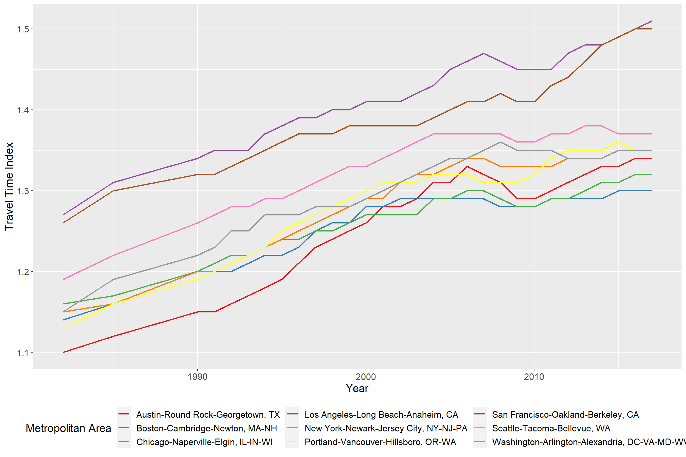
Figure 3: Travel Time Index by Metro Area (1982-2017)
Replica: Travel to Work/School Rate over 2020
Now we turn to the Replica data – how have work/school travel rates on the average weekday changed over 2020 in each metro area?
First, we load in all the replica data and bind it into one dataframe (from multiple CSV files).
#Replica data
replica_files = list.files('data/replica/')

replica_list = list()

for(i in 1:length(replica_files)){
  fh = replica_files[i]
  raw = read_csv(paste0('data/replica/',fh))
  replica_list[[i]] = raw
}

replica_frame = bind_rows(replica_list) %>%
  mutate(week_starting = as.Date(week_starting,
                                 format = '%m-%d-%Y'))
Then, we can plot the proportion of each metro area population traveling to work/school on the average weekday.
ggplot(replica_frame,aes(x=week_starting,y=traveling_work_school_proportion_avg_weekday,
                         color=msa,group=msa))+
  geom_line(size=0.8)+
  scale_y_continuous(labels=percent,limits = c(0,0.5))+
  scale_color_brewer(palette = 'Set1',name='Metropolitan Area')+
  ylab('Proportion of Metro Area Population\nTraveling to Work/School on Average Weekday')+
  xlab('Date (first day of week)')+
  theme(legend.position = 'bottom',
        text = element_text(size=14))+
  guides(color = guide_legend(nrow = 3))
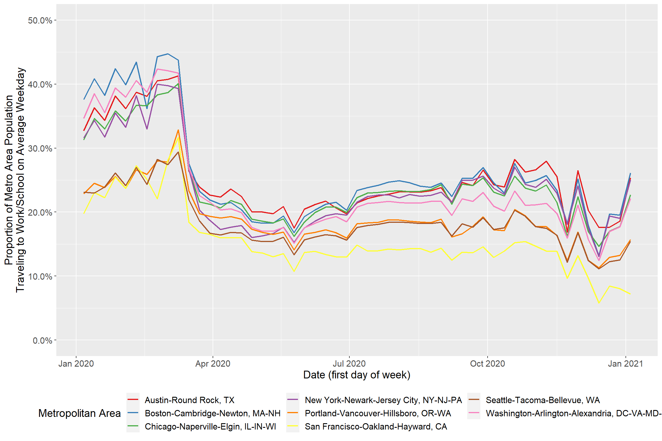
Figure 4: Proportion of Metro Area Population Traveling to Work/School on Average Weekday
To understand how we will adjust the travel time index, we normalize to a baseline, which we assume to be the first full week (post new years) in January 2020 – you can see how the proportion of people who travel to work/school changes relative to that baseline. Below, we will adjust the 2017 travel time index for each metro are based on the changes relative to that baseline.
ggplot(replica_frame,aes(x=week_starting,y=traveling_work_school_change_in_proportion_since_baseline,
                         color=msa,group=msa))+
  geom_line(size=0.8)+
  scale_y_continuous(labels=percent,limits = c(-0.75,0.75))+
  ylab('% Difference from Baseline of Work/School Travel on Average Weekday')+
  xlab('Date (first day of week)')+
  scale_color_brewer(palette = 'Set1',name='Metropolitan Area')+
  theme(legend.position = 'bottom',
        text = element_text(size=14))+
  guides(color = guide_legend(nrow = 3))
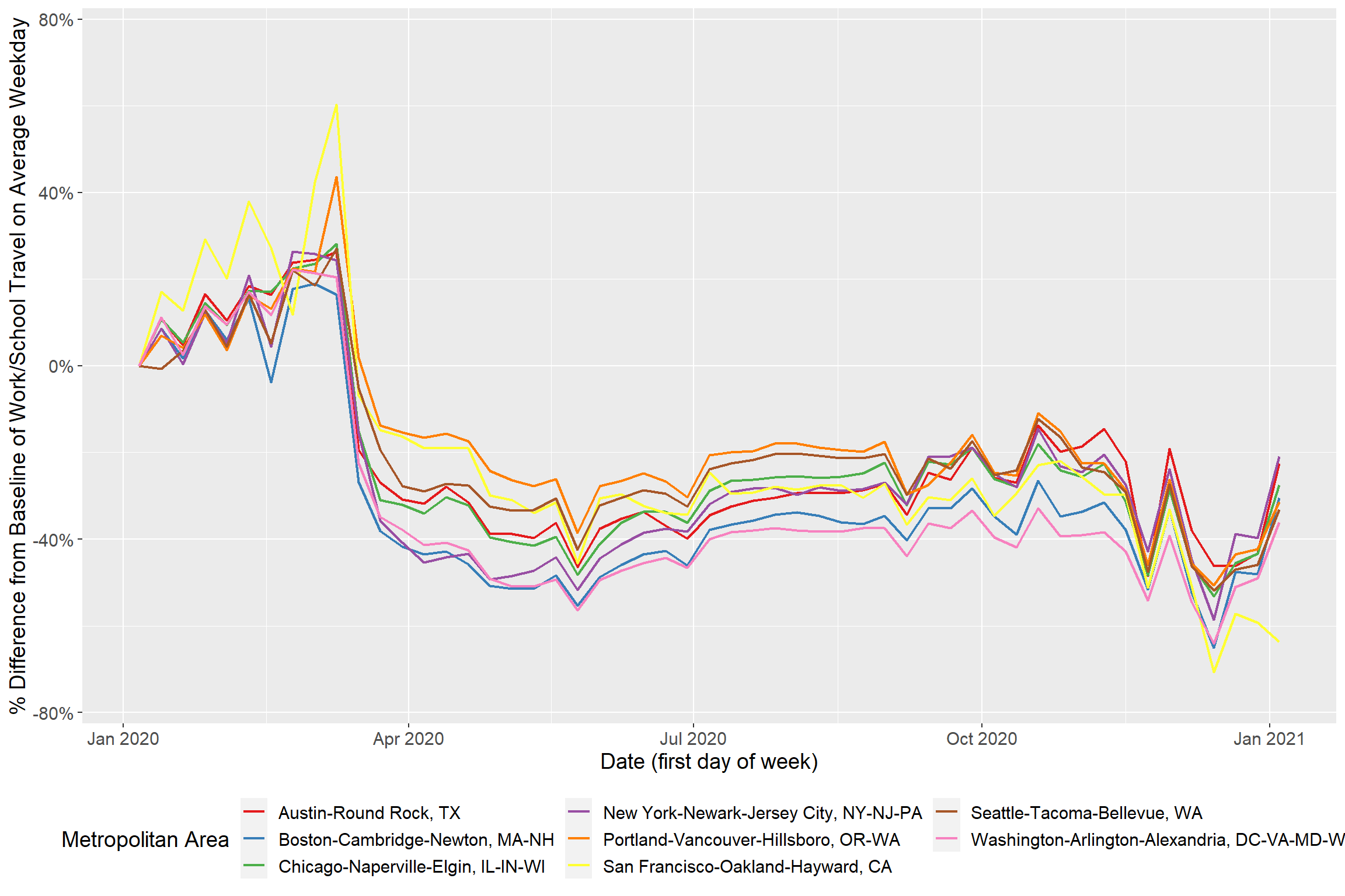
Figure 5: % Difference from Baseline of Work/School Travel on Average Weekday
Using Replica to Predict Present/Future Travel Time Indices
As described above, we can adjust the travel time indices for each metro area based on the change in proportion of travel to work/school. Below we have assumed that the travel time index cannot drop below 1, and so the proportion is only used to adjust the delta above 1.
adj_tt_index = sub_tt_index %>%
  filter(year == 2017) %>%
  left_join(replica_frame %>%
              select(geo_id,week_starting,traveling_work_school_change_in_proportion_since_baseline) %>%
              rename(GEOID = geo_id) %>%
              mutate(GEOID = as.character(GEOID))) %>%
  filter(!is.na(week_starting)) %>%
  mutate(ex_tti_delta = index - 1,
         prj_tti = ex_tti_delta*(1+traveling_work_school_change_in_proportion_since_baseline)+1) %>%
  mutate(adjustment_factor = prj_tti/index)

ggplot(adj_tt_index,aes(x=week_starting,y=prj_tti,
                        color=NAME,group=NAME, fill=NAME))+
  geom_point()+
  geom_smooth(lty=2,span=0.5)+
  theme(legend.position = 'bottom',
        text = element_text(size=14))+
  scale_color_brewer(palette = 'Set1',name='Metropolitan Area')+
  scale_fill_brewer(palette = 'Set1',name='Metropolitan Area')+
  facet_wrap(~NAME)+
  xlab('Date (first day of week)') + ylab('Adjusted Travel Time Index for 2020')+
  guides(color = guide_legend(nrow = 3))+
  guides(fill = guide_legend(nrow = 3))
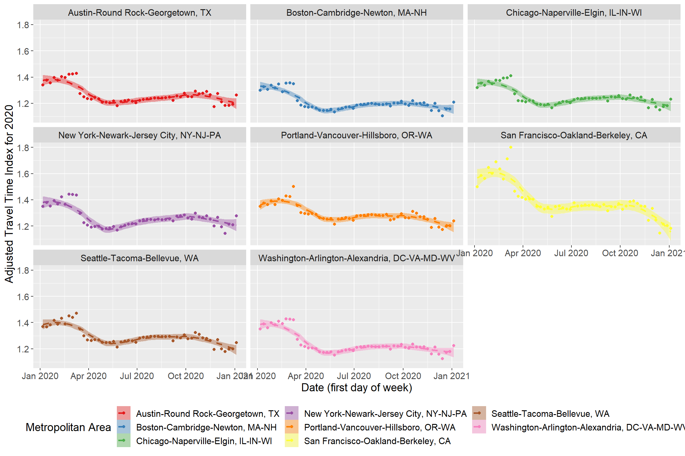
Figure 6: Adjusted Travel Time Indices for 2020
Example Travel Time Adjustment – Boston, MA
Below we demonstrate an example of using the adjustment factors calculated above to adjust travel times for a travel pattern in Boston – between Everett Square and Logan International Airport. First we compute the directions in both directions, similar to the way we did in the first example.
Directions to Logan
dir_results_to_logan = google_directions(origin = 'Everett Square, Boston, MA',
                  destination = 'Logan International Airport Boston, MA',
                  mode = 'driving',
                  departure_time = as.POSIXct('2021-02-23 07:30:00', tz='America/New_York'),
                  alternatives = TRUE)


tt_frame_to_logan = dir_results_to_logan$routes$legs %>%
  tibble(legs = .) %>%
  mutate(alternative_num = 1:n()) %>%
  unnest(legs) %>%
  select(alternative_num,contains('duration')) %>%
  mutate(duration_minutes_no_traffic = duration$value/60,
         duration_minutes_with_traffic = duration_in_traffic$value/60) %>%
  select(alternative_num,duration_minutes_no_traffic,duration_minutes_with_traffic)

polys_to_logan = dir_results_to_logan$routes$overview_polyline$points %>%
  tibble(poly=.) %>%
  mutate(decoded_poly = map(poly,~decode_pl(.x))) %>%
  mutate(alternative_num = 1:n()) %>%
  left_join(tt_frame_to_logan) %>%
  mutate(map_label = paste0('Alternative #',alternative_num,': ',
                            round(duration_minutes_with_traffic,1),' minutes with traffic')) %>%
  mutate(tti = duration_minutes_with_traffic/duration_minutes_no_traffic) %>%
  filter(!is.na(tti))

#See what the travel time indices are
print(polys_to_logan$tti)
[1] 0.9043367 0.9193548 0.9208633google_map(data = polys_to_logan) %>%
add_polylines(polyline = 'poly',stroke_weight = 9,mouse_over = 'map_label')
Figure 7: Routes to Logan
Directions from Logan
dir_results_from_logan = google_directions(destination= 'Everett Square, Boston, MA',
                  origin = 'Logan International Airport Boston, MA',
                  mode = 'driving',
                  departure_time = as.POSIXct('2021-02-23 12:00:00', tz='America/New_York'),
                  alternatives = TRUE)


tt_frame_from_logan = dir_results_from_logan$routes$legs %>%
  tibble(legs = .) %>%
  mutate(alternative_num = 1:n()) %>%
  unnest(legs) %>%
  select(alternative_num,contains('duration')) %>%
  mutate(duration_minutes_no_traffic = duration$value/60,
         duration_minutes_with_traffic = duration_in_traffic$value/60) %>%
  select(alternative_num,duration_minutes_no_traffic,duration_minutes_with_traffic)

polys_from_logan = dir_results_to_logan$routes$overview_polyline$points %>%
  tibble(poly=.) %>%
  mutate(decoded_poly = map(poly,~decode_pl(.x))) %>%
  mutate(alternative_num = 1:n()) %>%
  left_join(tt_frame_from_logan) %>%
  mutate(map_label = paste0('Alternative #',alternative_num,': ',
                            round(duration_minutes_with_traffic,1),' minutes with traffic')) %>%
  mutate(tti = duration_minutes_with_traffic/duration_minutes_no_traffic) %>%
  filter(!is.na(tti))

#See what the travel time indices are
print(polys_from_logan$tti)
[1] 0.8807692 0.9112769google_map(data = polys_from_logan) %>%
add_polylines(polyline = 'poly',stroke_weight = 9,mouse_over = 'map_label')
Figure 8: Routes from Logan
Adjusting Travel Times
We then grab the relevant adjustment factor from the above calculation – we assume the adjustment factor in Boston calculated for the week starting 2021-01-04 will give us an idea of how different the traffic is on a weekday in January from pre-pandemic levels. We then use that adjustment factor to scale up the travel times (without traffic) we got from Google. You can see below that the factor used (in this case we divided by 0.93) gets us a higher travel time than computed by Google with traffic – this speaks to the ahistorical level of traffic congestion occuring the COVID-19 pandemic. Both the Texas Transportation Institute numbers and the Replica numbers used are averages for a metro area, and so Google’s data may be more localized than these factors allow us to get. Professional judgment should be used with these estimates – I would use them more to provide a range of travel times to client, rather than a precise prediction.
boston_adj_factor = adj_tt_index %>%
  filter(urban_area=='Boston, MA-NH-RI') %>%
  tail(1) %>%
  pull(adjustment_factor)

print(boston_adj_factor)
[1] 0.9296703bound_travel_times = bind_rows(
polys_from_logan %>%
select(alternative_num,duration_minutes_no_traffic,duration_minutes_with_traffic) %>%
mutate(direction = 'From Logan, 12 PM'),
polys_to_logan %>%
select(alternative_num,duration_minutes_no_traffic,duration_minutes_with_traffic) %>%
mutate(direction = 'To Logan, 7:30 AM')
) %>%
mutate(adj_traffic_time = duration_minutes_no_traffic/boston_adj_factor) %>%
pivot_longer(cols = c(duration_minutes_no_traffic,duration_minutes_with_traffic,
adj_traffic_time)) %>%
left_join(tibble(
name = c('duration_minutes_no_traffic',
'duration_minutes_with_traffic',
'adj_traffic_time'),
plot_label = c('Google Duration, No Traffic',
'Google Duration, With Traffic',
'Adjusted Duration assuming pre-pandemic traffic')
)) %>%
mutate(direction = factor(direction,ordered=TRUE,
levels = c('To Logan, 7:30 AM','From Logan, 12 PM')),
plot_label = factor(plot_label,ordered=TRUE,
levels = c('Google Duration, No Traffic',
'Google Duration, With Traffic',
'Adjusted Duration assuming pre-pandemic traffic')))
ggplot(bound_travel_times,aes(x=factor(alternative_num),y=value,fill=plot_label))+
geom_col(position = position_dodge())+
geom_label(aes(label=round(value,1)),position = position_dodge(width=0.9),color='white',
fontface='bold', show.legend = FALSE)+
facet_wrap(~direction,nrow=1)+
scale_fill_brewer(palette = 'Set1')+
xlab('Route Alternative')+
ylab('Travel Time (minutes)')+
theme(legend.position = 'bottom', text = element_text(size=14))+
guides(fill = guide_legend(nrow=3,title = 'Estimate Type'))
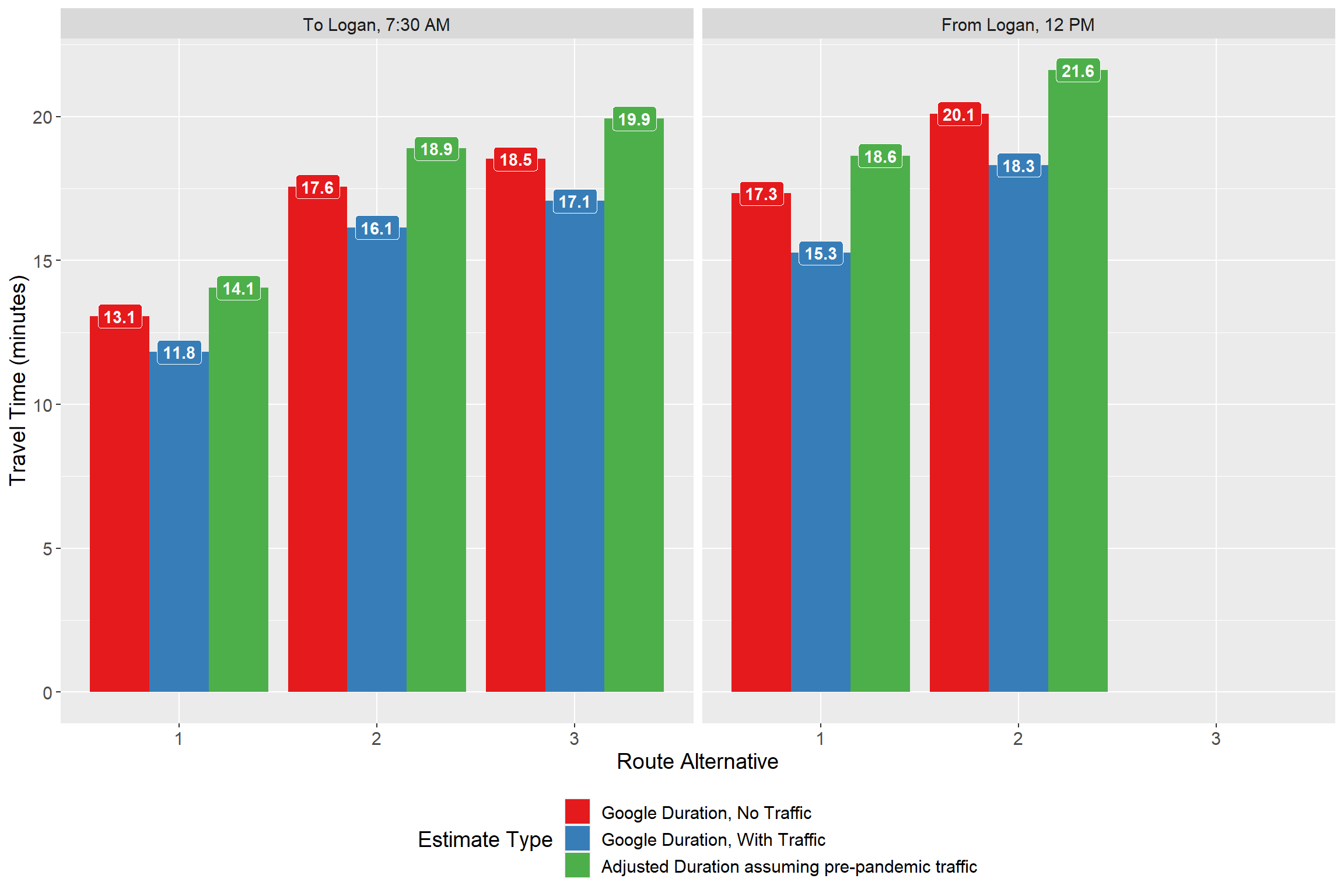
Figure 9: Example Adjusted Travel Times in Boston
This content was presented to Nelson\Nygaard Staff at a Lunch and Learn webinar on Thursday, January 21st, and is available as a recording here and embedded at the top of the page.