This content was presented to Nelson\Nygaard Staff at a Lunch and Learn webinar on Friday, September 17th, 2020, and is available as a recording here and embedded below.
Introduction
Today we are going to be covering several data products provided by the U.S. Census Bureau that often in form all types of work we do at Nelson\Nygaard, and how R packages can be used to make querying, downloading, and aggregating that data easier. We will start by discussing census geographies themselves, which can be downloaded quickly with the tigris package. We will then make some queries of Census demographic data using the tidycensus package. We will end using the lehdr package to understand home-work flows. These are great tools for many different types of projects across the United States.
Census Geographies with tigris
Acknowledgment: This portion of this module heavily draws upon, including direct copy-paste of markdown content, the vignettes developed for the tigris package, available on the package documentation website.
Census data is provided to the public in several data products, but across all of them survey data is aggregated to both time (a paritcular year or a set of years) and place (a particular geographic area). You are likely already familiar with some census geographies. The basic breakdown of census geographies in the United States is as follows, by level of hierarchy: 1. Nation 2. State 3. County 4. Tract 5. Block group 6. Block
There are other aggregations of those units, such as divisions and regions, as well as geographies that are important but do not neccesarily align with county/tract boundaries, such as Census Designated Places (i.e. cities, towns, other types of municipalities, and unincorporated but ‘designated’ places). tigris helps you to download all of these geographies quickly into R as sf objects. tigris is called that because all census geographies comprise the TIGER data set, which stands for Topologically Integrated Geographic Encoding and Referencing. There are also linear geographies as well, such as roads, waterways, and rail lines. Typically it is preferred to use your respective city or MPO’s road network, because it will be better maintained for local characteristics, but sometimes TIGER is the only option! TIGER files are given a major update every ten years coinciding with the decennial census (the 2020 census is wrapping up soon). Below, the datasets available in TIGER (and likewise, tigris) are enumerated with their function name.
Available datasets:
Please note: cartographic boundary files in tigris are not available for 2011 and 2012.
| Function | Datasets available | Years available |
|---|---|---|
nation() |
cartographic (1:5m; 1:20m) | 2013-2019 |
divisions() |
cartographic (1:500k; 1:5m; 1:20m) | 2013-2019 |
regions() |
cartographic (1:500k; 1:5m; 1:20m) | 2013-2019 |
states() |
TIGER/Line; cartographic (1:500k; 1:5m; 1:20m) | 1990, 2000, 2010-2019 |
counties() |
TIGER/Line; cartographic (1:500k; 1:5m; 1:20m) | 1990, 2000, 2010-2019 |
tracts() |
TIGER/Line; cartographic (1:500k) | 1990, 2000, 2010-2019 |
block_groups() |
TIGER/Line; cartographic (1:500k) | 1990, 2000, 2010-2019 |
blocks() |
TIGER/Line | 2000, 2010-2019 |
places() |
TIGER/Line; cartographic (1:500k) | 2011-2019 |
pumas() |
TIGER/Line; cartographic (1:500k) | 2012-2019 |
school_districts() |
TIGER/Line; cartographic | 2011-2019 |
zctas() |
TIGER/Line; cartographic (1:500k) | 2000, 2010, 2012-2019 |
congressional_districts() |
TIGER/Line; cartographic (1:500k; 1:5m; 1:20m) | 2011-2019 |
state_legislative_districts() |
TIGER/Line; cartographic (1:500k) | 2011-2019 |
voting_districts() |
TIGER/Line | 2012 |
area_water() |
TIGER/Line | 2011-2019 |
linear_water() |
TIGER/Line | 2011-2019 |
coastline |
TIGER/Line() | 2013-2019 |
core_based_statistical_areas() |
TIGER/Line; cartographic (1:500k; 1:5m; 1:20m) | 2011-2019 |
combined_statistical_areas() |
TIGER/Line; cartographic (1:500k; 1:5m; 1:20m) | 2011-2019 |
metro_divisions() |
TIGER/Line | 2011-2019 |
new_england() |
TIGER/Line; cartographic (1:500k) | 2011-2019 |
county_subdivisions() |
TIGER/Line; cartographic (1:500k) | 2010-2019 |
urban_areas() |
TIGER/Line; cartographic (1:500k) | 2012-2019 |
primary_roads() |
TIGER/Line | 2011-2019 |
primary_secondary_roads() |
TIGER/Line | 2011-2019 |
roads() |
TIGER/Line | 2011-2019 |
rails() |
TIGER/Line | 2011-2019 |
native_areas() |
TIGER/Line; cartographic (1:500k) | 2011-2019 |
alaska_native_regional_corporations() |
TIGER/Line; cartographic (1:500k) | 2011-2019 |
tribal_block_groups() |
TIGER/Line | 2011-2019 |
tribal_census_tracts() |
TIGER/Line | 2011-2019 |
tribal_subdivisions_national() |
TIGER/Line | 2011-2019 |
landmarks() |
TIGER/Line | 2011-2019 |
military() |
TIGER/Line | 2011-2019 |
As of version 1.0 (released in July 2020), tigris functions return simple features objects with a default year of 2019. To get started, choose a function from the table above and use it with a state and/or county if required (this will result in a quicker download of a smaller file). You’ll get back an sf object for use in your mapping and spatial analysis projects.
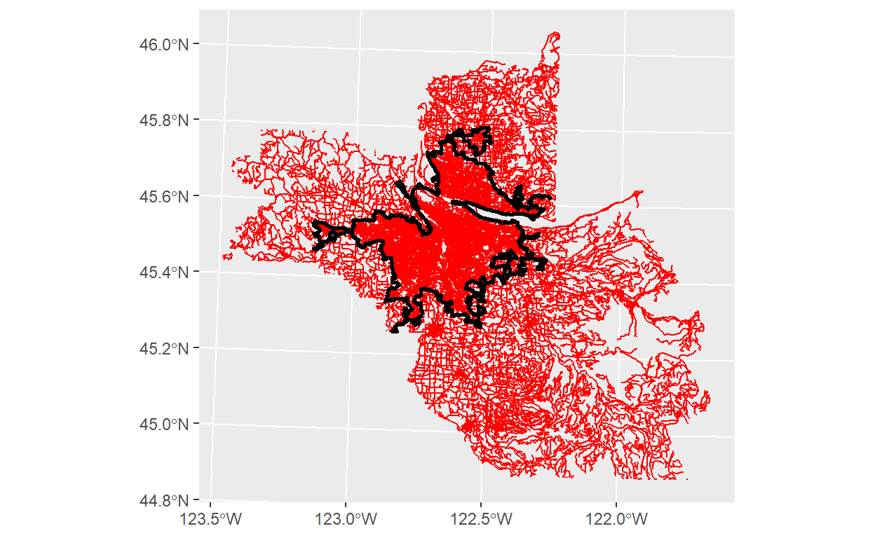
Here are some examples with some Portland metro area data - we are going to try to create a leaflet map with roads() and places() within the Portland metro area. We will define the Portland metro area based on the urban_areas() - for more on the Census’s definitions of urbanized and statistical areas, refer to this page.
Example - Part 1
library(tigris)
library(tidyverse)
library(sf)
library(leaflet)
library(stringr)
urb_areas = urban_areas()
head(urb_areas)
portland_urban_area = urb_areas %>%
filter(str_detect(NAME10,'Portland, OR')) %>%
st_transform(4326)
#Union, buffer, cast, and simlify all done here to try to remove vertices from boundary, making subsetting faster (but not as precise)
simp_pdx_ua = portland_urban_area %>%
st_transform(2269) %>%
st_union() %>%
st_buffer(1) %>%
st_cast('POLYGON') %>%
st_simplify()
#Have to query these objects by state and county separately
or_roads = roads(state='OR',county = c('Multnomah','Washington','Clackamas')) %>%
st_transform(4326)
wa_roads = roads(state='WA',county = c('Clark')) %>%
st_transform(4326)
#Binding sf objects is still a little wonky - have to reassert as sf column and object
bound_roads = bind_rows(
or_roads %>% as_tibble(),
wa_roads %>% as_tibble()
) %>%
mutate(geometry = st_sfc(geometry,crs=4326)) %>%
st_as_sf() %>%
st_transform(2269)
#This will take 30 seconds or so, road data is big!
ggplot()+
geom_sf(data = bound_roads,color='red')+
geom_sf(data = simp_pdx_ua,color='black',size=1,
#Want to have no fill to see roads through polygon
fill=NA)
#I was going to do the intersection with the actual boundaries, but it was taking a few minutes, so not great for an example. You can do on your own! I did with the convex hull instead.
# sub_bound_roads = bound_roads %>%
# st_intersection(simp_pdx_ua)
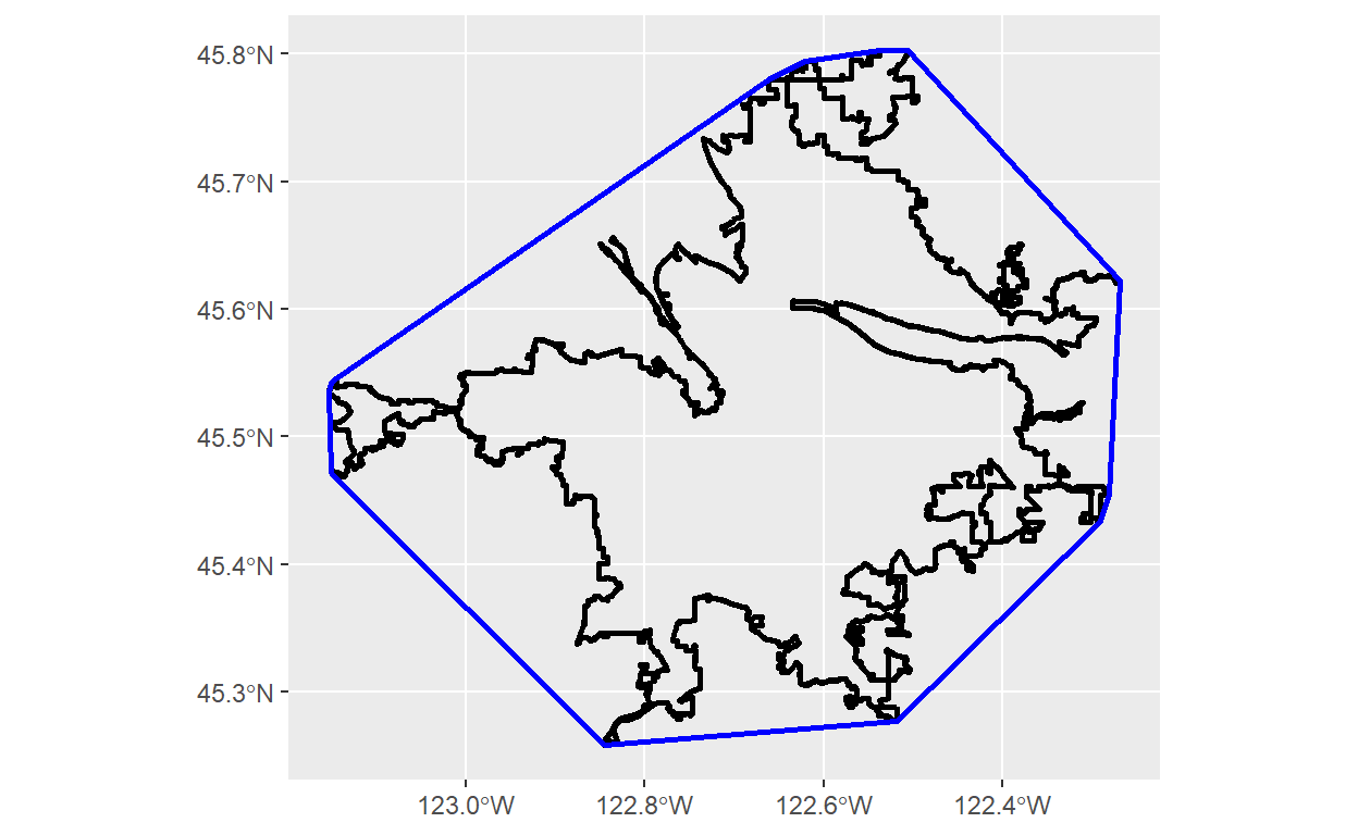
#Sometimes if you are doing complex spatial subsetting, you can speed it up using convex hulls
pdx_hull = portland_urban_area %>%
st_transform(2269) %>%
st_convex_hull()
#Here is what a convex hull looks like
ggplot()+
geom_sf(data = portland_urban_area,color='black',size=1,
#Want to have no fill to see roads through polygon
fill=NA)+
geom_sf(data= pdx_hull,color='blue',size=1,fill=NA)
#Codebook for MTFCC feature in TIGER geographies here: https://www2.census.gov/geo/pdfs/reference/mtfccs2019.pdf
big_roads = bound_roads %>%
filter(MTFCC %in% c('S1100', #Primary roads
'S1200')) %>% #Secondary roads
st_cast('LINESTRING') %>%
st_intersection(pdx_hull %>%
select(geometry)) %>%
mutate(sf_type = map_chr(geometry,~class(.x)[2])) %>%
filter(sf_type=='LINESTRING') %>%
st_cast('LINESTRING')
#Grab Places to subset as well
orwa_places = places(state=c('OR','WA'))
pdx_places = orwa_places %>%
st_transform(2269) %>%
st_intersection(simp_pdx_ua)
leaflet() %>%
addProviderTiles('CartoDB.Positron') %>%
#You can put a polygon on a leaflet map as a polyline to only show boundary and not area
addPolylines(data = simp_pdx_ua %>% st_transform(4326),
color='black',weight=2) %>%
addPolygons(data = pdx_places %>% st_transform(4326),
fillColor='red',fillOpacity = 0.5,color='white',
weight=1,label=~NAMELSAD,
#Highlight options helpful when you have overlapping objects
highlightOptions = highlightOptions(weight=3,sendToBack = TRUE,
fillOpacity = 0.8)) %>%
addPolylines(data=big_roads %>% st_transform(4326),
color='blue',weight=~ifelse(MTFCC=='S1200',4,2),
label=~FULLNAME)
Census Data Querying with tidycensus
Acknowledgment: This portion of this module heavily draws upon, including direct copy-paste of markdown content, the vignettes developed for the tidycensus package, available on the package documentation website.
Most of the time you are not using census geographies for the sole purpose of mapping the geographies themselves – these geographies are tied to a wealth of statistics available from the U.S. Census Bureau. The product NN uses most often from the U.S. Census Bureau is the American Community Survey – an annual sample survey (a statistically representative sub-sample of the population) conducted with a much more detailed survey than the Census itself (conducted on the entire U.S. population). We typically use the 5-year version, which pools samples from the previous 5 years on a rolling basis to achieve higher accuracy. The 1-year version has a smaller sample to work with so has a larger margin of error, but allows for understanding changes in trends at a higher temporal resolution. For demographic mapping, we generally recommend using the 5-year version.
Basic Usage
To get started working with tidycensus, users should load the package along with the tidyverse package, and set their Census API key. A key can be obtained from http://api.census.gov/data/key_signup.html.
library(tidycensus)
library(tidyverse)
census_api_key("04976a4a378107d2fb53acdbde84d0aad121cb10")
There are two major functions implemented in tidycensus: get_decennial(), which grants access to the 1990, 2000, and 2010 decennial US Census APIs, and get_acs(), which grants access to the 5-year American Community Survey APIs. As mentioned, we will be focusing on get_acs.
Searching for variables
Getting variables from the Census or ACS requires knowing the variable ID - and there are thousands of these IDs across the different Census files. To rapidly search for variables, use the load_variables() function. The function takes two required arguments: the year of the Census or endyear of the ACS sample, and the dataset - one of "sf1", "sf3", or "acs5". For ideal functionality, I recommend assigning the result of this function to a variable, setting cache = TRUE to store the result on your computer for future access, and using the View function in RStudio to interactively browse for variables.
v17 <- load_variables(2017, "acs5")
View(v17)
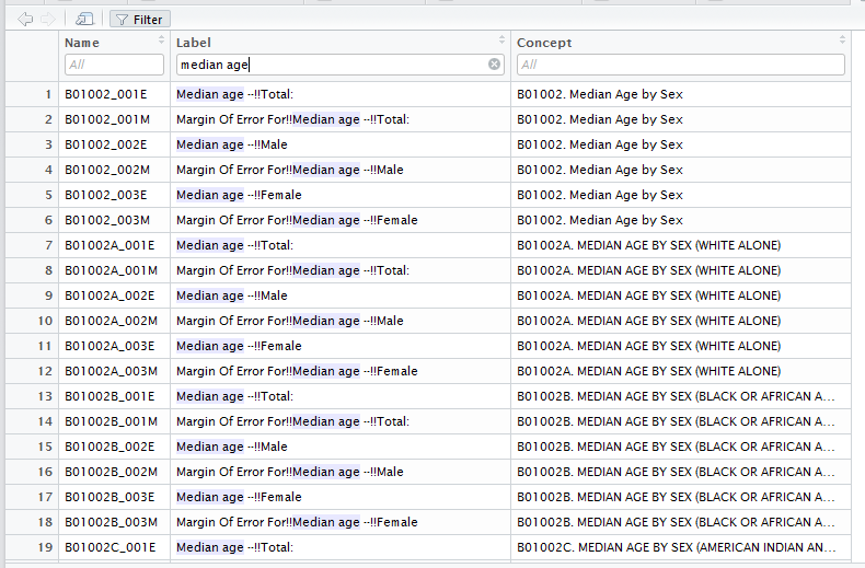
By filtering for “median age” I can quickly view the variable IDs that correspond to my query.
Working with ACS data
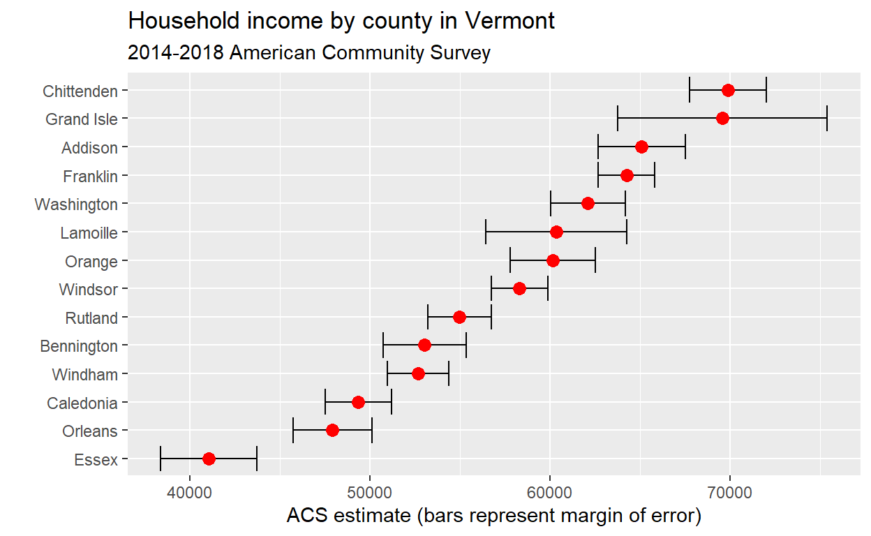
American Community Survey data differ from decennial Census data in that ACS data are based on an annual sample of approximately 3 million households, rather than a more complete enumeration of the US population. In turn, ACS data points are estimates characterized by a margin of error. tidycensus will always return the estimate and margin of error together for any requested variables when using get_acs(). In turn, when requesting ACS data with tidycensus, it is not necessary to specify the "E" or "M" suffix for a variable name. Let’s fetch median household income data from the 2014-2018 ACS for counties in Vermont.
The output of get_acs returns estimate and moe columns for the ACS estimate and margin of error, respectively. moe represents the default 90 percent confidence level around the estimate; this can be changed to 95 or 99 percent with the moe_level parameter in get_acs if desired. As we have the margin of error, we can visualize the uncertainty around the estimate:
vt %>%
mutate(NAME = gsub(" County, Vermont", "", NAME)) %>%
ggplot(aes(x = estimate, y = reorder(NAME, estimate))) +
geom_errorbarh(aes(xmin = estimate - moe, xmax = estimate + moe)) +
geom_point(color = "red", size = 3) +
labs(title = "Household income by county in Vermont",
subtitle = "2014-2018 American Community Survey",
y = "",
x = "ACS estimate (bars represent margin of error)")
Adding Geometry
If requested, tidycensus can return simple feature geometry for geographic units along with variables from the decennial US Census or American Community survey. By setting geometry = TRUE in a tidycensus function call, tidycensus will use the tigris package to retrieve the corresponding geographic dataset from the US Census Bureau and pre-merge it with the tabular data obtained from the Census API. As of tidycensus version 0.9.9.2, geometry = TRUE is supported for all geographies currently available in the package. Of course you can also just query the geographies yourself from tigris, and join data on the GEOID as needed.
The following example shows median household income from the 2014-2018 ACS for Census tracts in Orange County, California:
Our object orange looks much like the basic tidycensus output, but with a geometry list-column describing the geometry of each feature, using the geographic coordinate system NAD 1983 (EPSG: 4269) which is the default for Census shapefiles. tidycensus uses the Census cartographic boundary shapefiles for faster processing; if you prefer the TIGER/Line shapefiles, set cb = FALSE in the function call.
As the dataset is in a tidy format, it can be quickly visualized with the geom_sf functionality currently in the development version of ggplot2:
orange %>%
ggplot(aes(fill = estimate)) +
geom_sf(color = NA) +
coord_sf(crs = 26911) +
scale_fill_viridis_c(option = "magma")
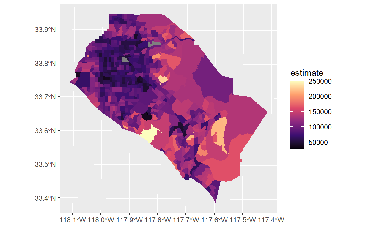
Please note that the UTM Zone 11N coordinate system (26911) is appropriate for Southern California but may not be for your area of interest.
Example - Part 2
Let’s try to map the median income of all of the CDPs we mapped in the first part of this module.
library(scales)
pdx_cdp_med_income = get_acs(state=c('OR','WA'),geography = 'place',
variables = c(medincome = "B19013_001")) %>%
#Filtering for GEOIDs in PDX Places
filter(GEOID %in% pdx_places$GEOID)
#Joining ACS data to shape
pdx_cdp_mi_shape = pdx_places %>%
left_join(pdx_cdp_med_income %>%
select(GEOID,estimate))
income_pal = colorNumeric(
#Scales package lets you access color brewer palettes
palette = brewer_pal(palette = 'Greens')(5),
domain = pdx_cdp_mi_shape$estimate
)
leaflet() %>%
addProviderTiles('CartoDB.Positron') %>%
#You can put a polygon on a leaflet map as a polyline to only show boundary and not area
addPolylines(data = simp_pdx_ua %>% st_transform(4326),
color='black',weight=2) %>%
addPolygons(data = pdx_cdp_mi_shape %>% st_transform(4326),
fillColor=~income_pal(estimate),fillOpacity = 0.5,color='white',
weight=1,label=~paste0(NAMELSAD,': ',dollar(estimate)),
highlightOptions = highlightOptions(weight=3,sendToBack = TRUE,
fillOpacity = 0.8)) %>%
addLegend(pal = income_pal,values =pdx_cdp_mi_shape$estimate,
labFormat = labelFormat(prefix = '$'),title = 'Median<br>Household<br>Income')
Downloading and Aggregating LODES data with lehdr
Acknowledgment: This portion of this module heavily draws upon, including direct copy-paste of markdown content, the vignettes developed for the lehdr package, available on the package documentation website.
In addition the residential-based statistics the U.S. Census Bureau provides through ACS (and the Census itself), another annual data product they offer is the Longitudinal Employer Household Dynamics (LEHD) Origin Destination Employment Statistics (LODES, for short!) data set. There are other LEHD data products offered that do not yet appear to have an R wrapper, but the package we will be looking at (lehdr) is in development.
The LODES data set is based on survey data as well as residential location data (from the ACS and the Census) and workplace location data that the Census Bureau and the Bureau of Labor Statistics (BLS) collect. It is often used in work at NN to understand employment locations as well as origin-destination patterns between home locations and employment locations. As it is a national data set, it is not as well attuned to local dynamics as the local MPO would be in their travel surveying efforts, so I would always defer to recent travel survey and modeling data from an MPO if that is available. That said, LODES is a great product for where there is no travel survey coverage, or a travel survey has not been conducted in some time. It is provided at the Census Block level, and so as you can guess the datasets can get pretty large! Which can make Excel a bit clunky for the job depending on the area you are looking at, but R has no problem handling!
Installation
lehdr has not yet been submitted to CRAN so installing using devtools is required.
install.packages('devtools')
devtools::install_github("jamgreen/lehdr")
Usage
This first example pulls the Oregon (state = "or") 2014 (year = 2014), origin-destination (lodes_type = "od"), all jobs including private primary, secondary, and Federal (job_type = "JT01"), all jobs across ages, earnings, and industry (segment = "S000"), aggregated at the Census Tract level rather than the default Census Block (agg_geo = "tract").
Note: LODES data is large, so some of these steps will take a minute or more to run.
or_od <- grab_lodes(state = "or", year = 2014, lodes_type = "od", job_type = "JT01",
segment = "S000", state_part = "main", agg_geo = "tract")
head(or_od)
# A tibble: 6 x 14
year state w_tract h_tract S000 SA01 SA02 SA03 SE01 SE02
<dbl> <chr> <chr> <chr> <dbl> <dbl> <dbl> <dbl> <dbl> <dbl>
1 2014 OR 410019501~ 41001950~ 89 6 37 46 35 30
2 2014 OR 410019501~ 41001950~ 35 2 25 8 6 13
3 2014 OR 410019501~ 41001950~ 23 6 12 5 5 12
4 2014 OR 410019501~ 41001950~ 20 0 17 3 4 4
5 2014 OR 410019501~ 41001950~ 24 8 10 6 3 12
6 2014 OR 410019501~ 41001950~ 10 3 5 2 4 5
# ... with 4 more variables: SE03 <dbl>, SI01 <dbl>, SI02 <dbl>,
# SI03 <dbl>The package can be used to retrieve multiple states and years at the same time by creating a vector or list. This second example pulls the Oregon AND Rhode Island (state = c("or", "ri")) for 2013 and 2014 (year = c(2013, 2014) or year = 2013:2014).
or_ri_od <- grab_lodes(state = c("or", "ri"), year = c(2013, 2014),
lodes_type = "od", job_type = "JT01",
segment = "S000", state_part = "main", agg_geo = "tract")
head(or_ri_od)
# A tibble: 6 x 14
year state w_tract h_tract S000 SA01 SA02 SA03 SE01 SE02
<chr> <chr> <chr> <chr> <dbl> <dbl> <dbl> <dbl> <dbl> <dbl>
1 2013 OR 410019501~ 41001950~ 80 4 39 37 25 30
2 2013 OR 410019501~ 41001950~ 27 4 15 8 8 11
3 2013 OR 410019501~ 41001950~ 11 1 5 5 6 3
4 2013 OR 410019501~ 41001950~ 21 3 14 4 5 8
5 2013 OR 410019501~ 41001950~ 27 12 8 7 4 15
6 2013 OR 410019501~ 41001950~ 4 1 2 1 2 0
# ... with 4 more variables: SE03 <dbl>, SI01 <dbl>, SI02 <dbl>,
# SI03 <dbl>Not all years are available for each state. To see all options for lodes_type, job_type, and segment and the availability for each state/year, please see the most recent LEHD Technical Document at https://lehd.ces.census.gov/data/lodes/LODES7/.
Other common uses might include retrieving Residential or Work Area Characteristics (lodes_type = "rac" or lodes_type = "wac" respectively), low income jobs (segment = "SE01") or good producing jobs (segment = "SI01"). Other common geographies might include retrieving data at the Census Block level (agg_geo = "block", not necessary as it is default) – but see below for other aggregation levels.
Additional Examples
Adding at County level signifiers
The following examples loads work area characteristics (wac), then uses the work area geoidw_geocode to create a variable that is just the county w_county_fips. Similar transformations can be made on residence area characteristics (rac) by using the h_geocode variable. Both variables are available in origin-destination (od) datasets and with od, one would need to set a h_county_fips and on w_county_fips.
md_rac <- grab_lodes(state = "md", year = 2015, lodes_type = "wac", job_type = "JT01", segment = "S000")
head(md_rac)
# A tibble: 6 x 55
w_geocode C000 CA01 CA02 CA03 CE01 CE02 CE03 CNS01 CNS02
<chr> <dbl> <dbl> <dbl> <dbl> <dbl> <dbl> <dbl> <dbl> <dbl>
1 2400100010010~ 7 3 3 1 4 3 0 0 0
2 2400100010010~ 1 0 1 0 0 1 0 0 0
3 2400100010010~ 10 2 3 5 7 3 0 0 0
4 2400100010011~ 2 0 2 0 0 1 1 0 0
5 2400100010020~ 8 4 4 0 7 1 0 0 0
6 2400100010020~ 2 0 2 0 0 2 0 0 0
# ... with 45 more variables: CNS03 <dbl>, CNS04 <dbl>, CNS05 <dbl>,
# CNS06 <dbl>, CNS07 <dbl>, CNS08 <dbl>, CNS09 <dbl>, CNS10 <dbl>,
# CNS11 <dbl>, CNS12 <dbl>, CNS13 <dbl>, CNS14 <dbl>, CNS15 <dbl>,
# CNS16 <dbl>, CNS17 <dbl>, CNS18 <dbl>, CNS19 <dbl>, CNS20 <dbl>,
# CR01 <dbl>, CR02 <dbl>, CR03 <dbl>, CR04 <dbl>, CR05 <dbl>,
# CR07 <dbl>, CT01 <dbl>, CT02 <dbl>, CD01 <dbl>, CD02 <dbl>,
# CD03 <dbl>, CD04 <dbl>, CS01 <dbl>, CS02 <dbl>, CFA01 <dbl>,
# CFA02 <dbl>, CFA03 <dbl>, CFA04 <dbl>, CFA05 <dbl>, CFS01 <dbl>,
# CFS02 <dbl>, CFS03 <dbl>, CFS04 <dbl>, CFS05 <dbl>,
# createdate <chr>, year <dbl>, state <chr># A tibble: 6 x 56
w_geocode C000 CA01 CA02 CA03 CE01 CE02 CE03 CNS01 CNS02
<chr> <dbl> <dbl> <dbl> <dbl> <dbl> <dbl> <dbl> <dbl> <dbl>
1 2400100010010~ 7 3 3 1 4 3 0 0 0
2 2400100010010~ 1 0 1 0 0 1 0 0 0
3 2400100010010~ 10 2 3 5 7 3 0 0 0
4 2400100010011~ 2 0 2 0 0 1 1 0 0
5 2400100010020~ 8 4 4 0 7 1 0 0 0
6 2400100010020~ 2 0 2 0 0 2 0 0 0
# ... with 46 more variables: CNS03 <dbl>, CNS04 <dbl>, CNS05 <dbl>,
# CNS06 <dbl>, CNS07 <dbl>, CNS08 <dbl>, CNS09 <dbl>, CNS10 <dbl>,
# CNS11 <dbl>, CNS12 <dbl>, CNS13 <dbl>, CNS14 <dbl>, CNS15 <dbl>,
# CNS16 <dbl>, CNS17 <dbl>, CNS18 <dbl>, CNS19 <dbl>, CNS20 <dbl>,
# CR01 <dbl>, CR02 <dbl>, CR03 <dbl>, CR04 <dbl>, CR05 <dbl>,
# CR07 <dbl>, CT01 <dbl>, CT02 <dbl>, CD01 <dbl>, CD02 <dbl>,
# CD03 <dbl>, CD04 <dbl>, CS01 <dbl>, CS02 <dbl>, CFA01 <dbl>,
# CFA02 <dbl>, CFA03 <dbl>, CFA04 <dbl>, CFA05 <dbl>, CFS01 <dbl>,
# CFS02 <dbl>, CFS03 <dbl>, CFS04 <dbl>, CFS05 <dbl>,
# createdate <chr>, year <dbl>, state <chr>, w_county_fips <chr>Aggregating at the County level
To aggregate at the county level, continuing the above example, we must also drop the original lock geoid w_geocode, group by our new variable w_county_fips and our existing variables year and createdate, then aggregate the remaining numeric variables.
md_rac_county <- md_rac %>% mutate(w_county_fips = str_sub(w_geocode, 1, 5)) %>%
select(-"w_geocode") %>%
group_by(w_county_fips, state, year, createdate) %>%
summarise_if(is.numeric, sum)
head(md_rac_county)
# A tibble: 6 x 55
# Groups: w_county_fips, state, year [6]
w_county_fips state year createdate C000 CA01 CA02 CA03 CE01
<chr> <chr> <dbl> <chr> <dbl> <dbl> <dbl> <dbl> <dbl>
1 24001 MD 2015 20190826 25887 5653 13801 6433 5938
2 24003 MD 2015 20190826 237881 57186 125917 54778 44280
3 24005 MD 2015 20190826 345823 82049 180737 83037 68082
4 24009 MD 2015 20190826 20063 5119 10381 4563 4539
5 24011 MD 2015 20190826 7939 1567 4179 2193 1346
6 24013 MD 2015 20190826 52618 13124 26078 13416 11985
# ... with 46 more variables: CE02 <dbl>, CE03 <dbl>, CNS01 <dbl>,
# CNS02 <dbl>, CNS03 <dbl>, CNS04 <dbl>, CNS05 <dbl>, CNS06 <dbl>,
# CNS07 <dbl>, CNS08 <dbl>, CNS09 <dbl>, CNS10 <dbl>, CNS11 <dbl>,
# CNS12 <dbl>, CNS13 <dbl>, CNS14 <dbl>, CNS15 <dbl>, CNS16 <dbl>,
# CNS17 <dbl>, CNS18 <dbl>, CNS19 <dbl>, CNS20 <dbl>, CR01 <dbl>,
# CR02 <dbl>, CR03 <dbl>, CR04 <dbl>, CR05 <dbl>, CR07 <dbl>,
# CT01 <dbl>, CT02 <dbl>, CD01 <dbl>, CD02 <dbl>, CD03 <dbl>,
# CD04 <dbl>, CS01 <dbl>, CS02 <dbl>, CFA01 <dbl>, CFA02 <dbl>,
# CFA03 <dbl>, CFA04 <dbl>, CFA05 <dbl>, CFS01 <dbl>, CFS02 <dbl>,
# CFS03 <dbl>, CFS04 <dbl>, CFS05 <dbl>Alternatively, this functionality is also built-in to the package and advisable for origin-destination grabs. Here include an argument to aggregate at the County level (agg_geo = "county"):
md_rac_county <- grab_lodes(state = "md", year = 2015, lodes_type = "rac", job_type = "JT01",
segment = "S000", agg_geo = "county")
head(md_rac_county)
# A tibble: 6 x 44
year state h_county C000 CA01 CA02 CA03 CE01 CE02 CE03
<dbl> <chr> <chr> <dbl> <dbl> <dbl> <dbl> <dbl> <dbl> <dbl>
1 2015 MD 24001 24683 5488 13029 6166 5598 10294 8791
2 2015 MD 24003 239454 51186 131373 56895 38476 63599 137379
3 2015 MD 24005 371927 79756 198239 93932 62678 112647 196602
4 2015 MD 24009 32868 7565 17830 7473 5643 9029 18196
5 2015 MD 24011 14935 3285 7827 3823 2800 5829 6306
6 2015 MD 24013 80257 17028 42594 20635 13427 21671 45159
# ... with 34 more variables: CNS01 <dbl>, CNS02 <dbl>, CNS03 <dbl>,
# CNS04 <dbl>, CNS05 <dbl>, CNS06 <dbl>, CNS07 <dbl>, CNS08 <dbl>,
# CNS09 <dbl>, CNS10 <dbl>, CNS11 <dbl>, CNS12 <dbl>, CNS13 <dbl>,
# CNS14 <dbl>, CNS15 <dbl>, CNS16 <dbl>, CNS17 <dbl>, CNS18 <dbl>,
# CNS19 <dbl>, CNS20 <dbl>, CR01 <dbl>, CR02 <dbl>, CR03 <dbl>,
# CR04 <dbl>, CR05 <dbl>, CR07 <dbl>, CT01 <dbl>, CT02 <dbl>,
# CD01 <dbl>, CD02 <dbl>, CD03 <dbl>, CD04 <dbl>, CS01 <dbl>,
# CS02 <dbl>Aggregating Origin-Destination
As mentioned above, aggregating origin-destination is built-in. This takes care of aggregation on both the h_geocode and w_geocode variables:
md_od_county <- grab_lodes(state = "md", year = 2015, lodes_type = "od", job_type = "JT01",
segment = "S000", agg_geo = "county", state_part = "main")
head(md_od_county)
# A tibble: 6 x 14
year state w_county h_county S000 SA01 SA02 SA03 SE01 SE02
<dbl> <chr> <chr> <chr> <dbl> <dbl> <dbl> <dbl> <dbl> <dbl>
1 2015 MD 24001 24001 16347 3533 8570 4244 3911 7249
2 2015 MD 24001 24003 171 48 78 45 53 51
3 2015 MD 24001 24005 272 68 140 64 73 92
4 2015 MD 24001 24009 29 13 8 8 15 7
5 2015 MD 24001 24011 9 1 7 1 2 3
6 2015 MD 24001 24013 74 22 41 11 24 22
# ... with 4 more variables: SE03 <dbl>, SI01 <dbl>, SI02 <dbl>,
# SI03 <dbl>Aggregating at Block Group, Tract, or State level
Similarly, built-in functions exist to group at Block Group, Tract, County, and State levels. County was demonstrated above. All require setting the agg_geo argument. This aggregation works for all three LODES types.
md_rac_bg <- grab_lodes(state = "md", year = 2015, lodes_type = "rac", job_type = "JT01",
segment = "S000", agg_geo = "bg")
head(md_rac_bg)
# A tibble: 6 x 44
year state h_bg C000 CA01 CA02 CA03 CE01 CE02 CE03 CNS01
<dbl> <chr> <chr> <dbl> <dbl> <dbl> <dbl> <dbl> <dbl> <dbl> <dbl>
1 2015 MD 2400100~ 251 56 126 69 51 103 97 2
2 2015 MD 2400100~ 452 90 242 120 91 183 178 3
3 2015 MD 2400100~ 341 71 191 79 74 150 117 1
4 2015 MD 2400100~ 294 51 157 86 52 124 118 1
5 2015 MD 2400100~ 352 66 196 90 78 134 140 1
6 2015 MD 2400100~ 550 119 286 145 105 244 201 1
# ... with 33 more variables: CNS02 <dbl>, CNS03 <dbl>, CNS04 <dbl>,
# CNS05 <dbl>, CNS06 <dbl>, CNS07 <dbl>, CNS08 <dbl>, CNS09 <dbl>,
# CNS10 <dbl>, CNS11 <dbl>, CNS12 <dbl>, CNS13 <dbl>, CNS14 <dbl>,
# CNS15 <dbl>, CNS16 <dbl>, CNS17 <dbl>, CNS18 <dbl>, CNS19 <dbl>,
# CNS20 <dbl>, CR01 <dbl>, CR02 <dbl>, CR03 <dbl>, CR04 <dbl>,
# CR05 <dbl>, CR07 <dbl>, CT01 <dbl>, CT02 <dbl>, CD01 <dbl>,
# CD02 <dbl>, CD03 <dbl>, CD04 <dbl>, CS01 <dbl>, CS02 <dbl>md_rac_tract <- grab_lodes(state = "md", year = 2015, lodes_type = "rac", job_type = "JT01",
segment = "S000", agg_geo = "tract")
head(md_rac_tract)
# A tibble: 6 x 44
year state h_tract C000 CA01 CA02 CA03 CE01 CE02 CE03 CNS01
<dbl> <chr> <chr> <dbl> <dbl> <dbl> <dbl> <dbl> <dbl> <dbl> <dbl>
1 2015 MD 2400100~ 1044 217 559 268 216 436 392 6
2 2015 MD 2400100~ 1196 236 639 321 235 502 459 3
3 2015 MD 2400100~ 945 206 493 246 225 395 325 3
4 2015 MD 2400100~ 1134 228 598 308 282 466 386 0
5 2015 MD 2400100~ 746 159 371 216 184 337 225 1
6 2015 MD 2400100~ 1091 265 573 253 261 459 371 1
# ... with 33 more variables: CNS02 <dbl>, CNS03 <dbl>, CNS04 <dbl>,
# CNS05 <dbl>, CNS06 <dbl>, CNS07 <dbl>, CNS08 <dbl>, CNS09 <dbl>,
# CNS10 <dbl>, CNS11 <dbl>, CNS12 <dbl>, CNS13 <dbl>, CNS14 <dbl>,
# CNS15 <dbl>, CNS16 <dbl>, CNS17 <dbl>, CNS18 <dbl>, CNS19 <dbl>,
# CNS20 <dbl>, CR01 <dbl>, CR02 <dbl>, CR03 <dbl>, CR04 <dbl>,
# CR05 <dbl>, CR07 <dbl>, CT01 <dbl>, CT02 <dbl>, CD01 <dbl>,
# CD02 <dbl>, CD03 <dbl>, CD04 <dbl>, CS01 <dbl>, CS02 <dbl>md_rac_state <- grab_lodes(state = "md", year = 2015, lodes_type = "rac", job_type = "JT01",
segment = "S000", agg_geo = "state")
head(md_rac_state)
# A tibble: 1 x 44
year state h_state C000 CA01 CA02 CA03 CE01 CE02 CE03
<dbl> <chr> <chr> <dbl> <dbl> <dbl> <dbl> <dbl> <dbl> <dbl>
1 2015 MD 24 2.53e6 536277 1.39e6 610456 418694 748393 1.37e6
# ... with 34 more variables: CNS01 <dbl>, CNS02 <dbl>, CNS03 <dbl>,
# CNS04 <dbl>, CNS05 <dbl>, CNS06 <dbl>, CNS07 <dbl>, CNS08 <dbl>,
# CNS09 <dbl>, CNS10 <dbl>, CNS11 <dbl>, CNS12 <dbl>, CNS13 <dbl>,
# CNS14 <dbl>, CNS15 <dbl>, CNS16 <dbl>, CNS17 <dbl>, CNS18 <dbl>,
# CNS19 <dbl>, CNS20 <dbl>, CR01 <dbl>, CR02 <dbl>, CR03 <dbl>,
# CR04 <dbl>, CR05 <dbl>, CR07 <dbl>, CT01 <dbl>, CT02 <dbl>,
# CD01 <dbl>, CD02 <dbl>, CD03 <dbl>, CD04 <dbl>, CS01 <dbl>,
# CS02 <dbl>Example - Part 3
Let’s try to use LODES to get the job flows between CDPs in the Portland regions. 2017 is the latest year available – it takes them a few years to put each release together. Unfortunately I noticed when putting this example together, lehdr which seems overall better documented and maintained, does not have a function to read the LODES crosswalk file. This is included in another LODES package and I actually wrote a version of this myself at one point. I filed a corresponding issue on the lehdr GitHub and will contribute if the author desires. The other package, lodes, will be loaded to use the read_xwalk() function.
library(lodes)
library(lehdr)
#Can only grab one state at a time right now
orwa_lodes =grab_lodes(state = c('or','wa'),year = 2017,lodes_type = 'od',
agg_geo = 'bg',segment = 'S000',state_part = c('aux')) %>%
bind_rows(grab_lodes(state = c('or','wa'),year = 2017,lodes_type = 'od',
agg_geo = 'bg',segment = 'S000',state_part = c('main')))
orwa_xwalk = bind_rows(
read_xwalk('or'),
read_xwalk('wa')
)
sub_xwalk = orwa_xwalk %>%
filter(stplc %in% pdx_places$GEOID) %>%
distinct(st,bgrp,stplc) %>%
#Need to have all codes as character to join properly
mutate_all(as.character)
agg_plc_lodes = orwa_lodes %>%
rename(total_jobs = `S000`) %>%
group_by(h_bg,w_bg) %>%
summarise(total_jobs = sum(total_jobs)) %>%
left_join(sub_xwalk %>%
rename(h_st = st,
h_bg = bgrp,
h_stplc=stplc)) %>%
left_join(sub_xwalk %>%
rename(w_st = st,
w_bg = bgrp,
w_stplc=stplc)) %>%
group_by(h_st,h_stplc,w_st,w_stplc) %>%
summarise(total_jobs = sum(total_jobs))
#Going to use centroids to draw OD lines
pdx_plc_cents = pdx_places %>%
st_centroid()
agg_plc_od_shp = agg_plc_lodes %>%
ungroup() %>%
filter(!is.na(h_stplc),!is.na(w_stplc),
#Filtering out where home and work are same location (no line to draw...)
h_stplc!=w_stplc) %>%
mutate(od_line = pmap(.l = list(h_stplc,w_stplc),
.f = function(h_stplc,w_stplc){
h_cent = pdx_plc_cents %>%
filter(GEOID == h_stplc)
w_cent = pdx_plc_cents %>%
filter(GEOID == w_stplc)
hw_line = bind_rows(
h_cent %>% st_coordinates() %>% as_tibble(),
w_cent %>% st_coordinates() %>% as_tibble()
) %>%
#Have to convert to matrix to coerce into linestring
as.matrix() %>%
st_linestring()
return(hw_line)
})) %>%
mutate(od_line = st_sfc(od_line,crs =2269)) %>%
st_as_sf() %>%
left_join(pdx_places %>%
as_tibble() %>%
select(GEOID,NAME) %>%
rename(h_stplc = GEOID,
home_place = NAME)) %>%
left_join(pdx_places %>%
as_tibble() %>%
select(GEOID,NAME) %>%
rename(w_stplc = GEOID,
work_place = NAME))
#Setting a weight multiplier so job flow can be visualized proportionally on leaflet map
max_job_flow = max(agg_plc_od_shp$total_jobs)
max_weight = 30
weight_mult = max_weight/max_job_flow
leaflet() %>%
addProviderTiles('CartoDB.Positron') %>%
addPolylines(data = simp_pdx_ua %>% st_transform(4326),
color='black',weight=2,group = 'Urban Area Boundary') %>%
addPolygons(data = pdx_places %>% st_transform(4326),
fillColor='green',fillOpacity = 0.5,color='white',
weight=1,label=~NAMELSAD,
highlightOptions = highlightOptions(weight=3,sendToBack = TRUE,
fillOpacity = 0.8),
group='Place Polygons') %>%
addPolylines(data=big_roads %>% st_transform(4326),
color='blue',weight=~ifelse(MTFCC=='S1200',4,2),
label=~FULLNAME,
group='Roads') %>%
addPolylines(data = agg_plc_od_shp %>% st_transform(4326),
color = 'red',weight =~ total_jobs * weight_mult,
label=~ paste0(home_place,' to ',work_place,': ',comma(total_jobs),' jobs'),
opacity = 0.5,
highlightOptions = highlightOptions(sendToBack = TRUE,opacity = 1),
group='Job Flows') %>%
addLayersControl(overlayGroups = c('Urban Area Boundary','Roads','Place Polygons','Job Flows'))
Reference Materials
Run Through the Example Code Yourself
You can run through the example yourself based on the example code and data, which you can get by cloning (or just downloading as a ZIP) the GitHub repository for this course and navigating to the topics_setup/05_census directory. There you will see example_code.R, and the raw Doodle results in the data folder.
Further Reading
- Analyzing the US Census with R, written by Kyle Walker, is expected shortly per the
tigrisGitHub page. Until then, there are a lot of videos and blog posts on the web!
Related DataCamp Courses
This content was presented to Nelson\Nygaard Staff at a Lunch and Learn webinar on Friday, September 17th, 2020, and is available as a recording here and embedded at the top of the page.